... The Programmer God ...
a Universe Simulation coded at the Planck scale
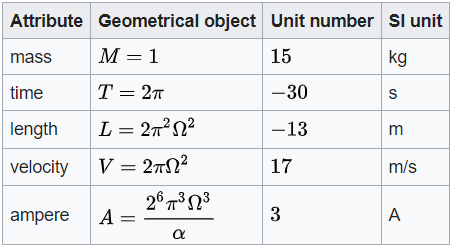
if we assign geometrical objects to mass, space and time,
and then link them via a unit number relationship,
we can build a physical universe from mathematical structures.
Could a Programmer God have used this approach?
The simulations mentioned in the article and on the wiki-site
are given here. The codes are written in C and python, C is faster and so better for long orbital radius and large center mass. I use codeblocks for my C compiler and Spyder for python but there are many online compilers. The codes here can be used under creative commons CC CC BY-NC-SA 4.0. This permits modifications to the code with attibution to the author. I used gnuplot for the animations and python for plots.
This page assumes that the reader is already familiar with the article and/or wiki page. The following sections refer to different aspects (2-body orbits, elliptical orbits, transition orbits ...), but the orbital section routine in each case is the same. I have separated simply them to keep the code readable.
The model is designed to represent events at the Planck scale and so the mathematics is simple but computationally intensive. The core concept behind this approach is that the universe does not require an external set of commands, rather it could be a geometrically autonomous computer; electrons orbit protons, not because of an external function (a set of pre-programmed rules as with our simulations), but due to geometrical imperatives, the respective geometries of the electron and proton leading to these orbits. The incremental expansion of the universe does the rest (as it expands it pulls the particles with it).
Variables (2-body orbits):
ipoints: number of points in the central mass (the Scwharzchild radius)
jpoints: total number of points (in a 2-body orbit, the orbiting point is 1 mass unit; jpoints = ipoints +1)
kr: sets orbital radius as multiples of ipoints (quantizes radius as a function of the Scwharzchild radius)
x[0], y[0]: start coordinates for the orbiting point
x[1], y[1]: start coordinates for the orbited mass center point (some simulations have x[1], y[1] and x[2], y[2]).
The Kepler derivation in Maple code format.
Note: the simulation itself doesn't distingush between points, they all rotate around each other and so the points may also be assigned random co-ordinates for complex orbits. The 2-body orbit is however the most convenient for comparison with real-world orbits. Comments and suggestions are welcome, the code is not optimized, further improvements to the averaging and orbital stability can be added but these must reflect the geometrical autonomy of the model.
1. 2-body orbits
The simulation (Gravitational-orbital-simulation-2body.c) simulates a single point orbiting a central mass. The calculated period and length of orbit are then compared with the simulation data to confirm that the calculation formulas do accurately represent the orbital data. Once this is established, these formulas can then be applied to simulating real world orbits. The earth-moon orbit is an example, as well as the Kepler derivation of G. Setting variable kr = 32 is probably the maximum radius for long double precision. Gnuplot can be used for animations.
Code at https://codingthecosmos.com/orbitals/nbody/
2. 2-body elliptical orbits
The simulation (gravitational-orbital-elliptical-orbits.cpp) is the same program as above but with an extra function, orbitals can travel either clock-wise or anti-clockwise. By choosing the ratio of clock-wise:anti-clockwise orbitals the degree of eccentricity can be controlled. The ratio 108:1 (kcurve = 108) gave an eccentricity close to Mercury.
Variables:
kcurve //0 = circular, 1 = straight line, 9999... = circular
direction //(1 anticlockwise, -1 = clockwise)
cycle //number of orbits to repeat
To extrapolate to mass = infinity for comparison with Mercury's orbit; Gravitational-orbital-ellipse-extrapolate.py was used.
Code at https://codingthecosmos.com/orbitals/ellipse/
3. Atomic orbitals
The 2-photon geometrical model is looked at here. The simulation (2-photon-gravitational-orbital-simulation.c) calculates a gravitational orbit albeit the rotation angle has been changed with the addition of an extra alpha term to accommodate the electron wave-state. There are several diagnostic programs included and a .gif simulation. I am working on the documentation.
Code at https://codingthecosmos.com/orbitals/atomic/
4. Orbital vs. Newton
A simple 3-body orbit was generated to compare this orbital model with a Newtonian generated orbit.
1. Newton-vs-Orbital_Orbital.py generates the data file data-3b-long.txt
2. Newton-vs-Orbital_Newton.py generates the corresponding orbit using the Newtonian leap-frog as shown in Newton-vs-Orbital-trajectory_comparison.png.
Code at https://codingthecosmos.com/orbitals/newton/