7. Geometric Origin of Quarks, the Mathematical Electron extended

Background

The mathematical electron model [2] represents the electron as a geometrical object described by the formula \(\psi\). Although dimensionless, this formula encodes the information required to characterize the physical electron parameters (wavelength, frequency, mass, charge) by embedding within its geometry the MLTA objects—analogues of Planck units for mass (\(m_P\)), length (\(l_p\)), time (\(t_p\)), and charge (\(A\)). The MLTA objects are themselves constructed from three fundamental numbers: the fine structure constant \(\alpha\), a mathematical constant \(\Omega\), and \(\pi\). This background is covered in depth in Article 6.

The electron formula \(\psi\) not only embeds these Planck objects but also dictates their frequency:

The electron wavelength and mass can then be given by:

Thus, the formula \(\psi\), which resembles the volume of a torus or surface of a 4-D hypersphere, is argued to be a complex geometry constructed from simpler MLTA geometries—and that these are natural Planck units.

Planck Objects MLTA

The base units MLTA are geometrical objects derived from two dimensionless constants: the fine structure constant \(\alpha\) and a mathematical constant \(\Omega\).

The inverse fine structure constant \(\alpha_{\text{inv}} = 137.035999139\) (CODATA 2014), and the constant \(\Omega\) has a potential solution in terms of \(\pi\) and \(e\):

The geometrical objects MLTVA are defined as follows:

Geometrical objects have the advantage over numbering systems given that their functions (attributes) can be embedded within their geometry. For example, the time object \(T\) embeds the function 'time', and the length object \(L\) embeds 'length'. These geometrical objects can then combine to form more complex objects, from electrons to macroscopic entities.

This requires a relationship between Planck unit geometries that defines how they may combine, represented by assigning to each attribute a unit number \(\theta\) based on a geometrical base-15 system (e.g., \(\theta = 15 \Leftrightarrow \text{kg}\)).

Since \(\alpha\) and \(\Omega\) can be assigned numerical values, the MLTA objects can be expressed numerically. These objects can be converted to their Planck unit equivalents by including dimensioned scalars. For example, \(V = 2\pi\Omega^2 = 25.3123819353\), and scalar \(v_{\text{SI}} = 11843707.905\) m/s gives \(c = V \cdot v_{\text{SI}} = 299792458\) m/s.

The scalar incorporates the dimension quantity and so is subject to the unit number relationship (the base-15 rule set), and so we then find that only two scalars are needed because in defined ratios they will overlap and cancel. For example:

Thus if we know any two scalars (\(\alpha\) and \(\Omega\) have fixed values), we can solve for the Planck units and subsequently for \(G\), \(h\), \(c\), \(e\), \(m_e\), \(k_B\).

For example, here we using scalars \(r\) (\(\theta = 8\)) and \(v\) (\(\theta = 17\)) to replace \(k, t, l, a\):

Mathematical Electron

The mathematical electron formula \(\psi\) incorporates dimensioned Planck units but is itself dimensionless (units = scalars = 1).

Electron Parameters

The electron parameters (mass, wavelength, frequency, charge) can be solved as the frequency of the Planck units themselves, which is \(\psi\). In SI units (from Table 4):

Electron wavelength \(\lambda_e = 2.4263102367 \times 10^{-12}\) m (CODATA 2014):

Electron mass \(m_e = 9.10938356 \times 10^{-31}\) kg (CODATA 2014):

Elementary charge \(e = 1.6021766208 \times 10^{-19}\) C (CODATA 2014):

Rydberg constant \(R = 10973731.568508\) m\(^{-1}\) (CODATA 2014):

These formulas show that wavelength is \(\psi\) units of Planck length, frequency is \(\psi\) units of Planck time, but electron mass is only 1 unit of Planck mass.

Summary: \(\psi\) encodes the physical electron

Article 6 demonstrated explicitly that the mathematical electron formula \(\psi = 2^{20}\pi^8 3^3 \alpha_{\mathrm{inv}}^3 \Omega^{15} = \frac{\sigma_e^3}{2\pi}\) contains exactly the information needed to reproduce all physical electron parameters. Here we summarise the result in a compact form, since it underlies all later sections of this article.

1. Mass: \(m_e = \frac{m_P}{\psi}\).
2. Wavelength: \(\lambda_e = 2\pi l_P\, \psi\).
3. Frequency: \(\nu_e = \frac{\psi}{t_P}\).
4. Charge: \(e = A T\), with \(A\) and \(T\) fixed by \(\alpha\) and \(\Omega\).

Thus all observable electron parameters \((m_e,\ \lambda_e,\ \nu_e,\ e)\) follow directly from the single invariant \(\psi=\frac{\sigma_e^3}{2\pi}\), which is the cubic monopole holonomy of the wave-state. Nothing beyond the MLTA geometrical objects \((M,L,T,A,V)\) and the constants \((\alpha,\Omega,\pi)\) is required, and these are all embedded within the formula for \(\psi\).

Point (mass) state versus wave (phase) state

Particle mass is a unit of Planck mass that occurs once per \(\psi\) units of Planck time, while other parameters are continuums of Planck units:

The electron is modelled not as a physical entity but rather as an oscillation between 2 distinct states; an electric wave-state (duration particle frequency) and a mass point-state (duration 1 unit of Planck time). At a given Planck time unit the electron occupies a point (mass) state of duration one Planck time \(t_P\). In this state the electron is dimensionless: the algebraic units in the formula (the \(\mathrm{AL}^3/T\) factors) cancel and no electric wave-state substructure is present. The point state therefore functions as a marker in the Planck-unit scaffolding of the universe rather than as a classical extended object. Immediately following the point state, the electron unfolds into a wave (phase) state of duration \(\tau_{\text{wave}} = \psi\, t_P\). During the wave state there is no intrinsic mass density: the physical degrees of freedom are purely topological phase units (the monopole amplitudes \(\sigma_e\)) whose non-abelian holonomy realizes \(\psi=\sigma_e^3/(2\pi)\). The electron's wavelength, spin and topological current are properties of this phase configuration; mass reappears only when the wave-state collapses back to the next Planck tick point state.

Quarks

Unit number rule

The charge on the electron derives from the embedded ampere \(A\) and length \(L\), while the electron formula \(\psi\) itself is dimensionless. These AL have the units for magnetic monopoles (ampere-meter) and appear analogous to quarks (3 monopoles per electron), but the perfect symmetry and stability of \(\psi\) provide no clear fracture point for electron disruption and so any internal electron structure would be from difficult to impossible to detect/measure.

The electron formula:

AL magnetic monopole: Here \(\psi\) is defined in terms of \(\sigma_e\), where AL is an ampere-meter (ampere-length = \(e \cdot c\), units for a magnetic monopole).

If the magnetic monopole \(\sigma_e\) could equate to a quark with electric charge \(-\frac{1}{3}e\), it would be an analogue of the D quark. Three D quarks would constitute the electron as DDD = (AL)×(AL)×(AL).

For the positron (anti-matter electron), we might expect the inverse charge, but AL units \(\theta = -10\), and no 'units \(\theta = +10\)' combination including A exists in the set of unit number relations. However, we can also derive our electron formula via a Planck temperature \(t_p\) AV monopole (ampere-velocity):

The units for \(\sigma_t\) unit number \(\theta = +20\), so if \(\theta = -10\) equates to \(-\frac{1}{3}e\), then \(\theta = +20\) might equate to \(+\frac{2}{3}e\), analogous to the U quark, the difference between them being a unit of time T (\(\theta = -30\)). The positron charge structure becomes DUU, resembling the proton's quark structure rather than simply being the electron's inverse. This could explain missing anti-matter and why proton and electron charge magnitudes match exactly.

Numerically: Adding proton (UUD) and electron (DDD) gives 2(UDD) = 20 - 10 - 10 = 0 (zero charge), scalars = 0. Converting between U and D via U & DDD (electron) = 20 - 10 - 10 - 10 = -10 (D), scalars = \(\frac{r^3}{v^2}\). The quark/monopoles themselves have physical units (the scalars have not cancelled) but experimental physics suggests that these combinations are unstable independent of other quarks.

Both DDD and DUU variations yield the same electron geometry and so in this respect the electron and positron are the same;

Particle Construction

Electron = ddd = \((AL)^3/T\) : \(\theta_e = 3(-10) = -30,\ q_e = -e\) ✓

Positron = duu : \(\theta_{e^+} = -10 + 2(20) = +30,\ q_{e^+} = +e\) ✓

Proton = DUU : \(\theta_p = 2(20) - 10 = +30,\ q_p = +e\) ✓

Neutron = UDD : \(\theta_n = 20 - 20 = 0,\ q_n = 0\) ✓

Observation: Positron and proton have identical \(\theta = +30\) and charge \(+e\), however the positron has independent quarks whereas the proton has complex quarks (the 1836× mass difference). From this we may premise that the electron and positron quarks are free (with minimum binding), but the proton and neutron quarks are significantly constrained (a complex internal structure). We cannot therefore directly compare these quarks as discrete units but we can reference both sets.

Photon as a neutral \(\Omega^{15}\) phase composite (low Kolmogorov complexity)

A key design goal of the MLTA framework is low descriptive complexity: new phenomena should be representable using the same small set of primitives \((\alpha,\Omega,\pi)\) and the same MLTA objects that already generate the electron invariant \(\psi\). Since we showed that the electron embeds quark-like monopole objects \(D=AL\) and \(U=AV\), the natural next question is whether the photon can be represented by a closely related internal structure, so that "the easiest thing to mix with water is more water": particles and photons would then share a common geometric substrate.

Monopole blocks carry the same \(\Omega^5\) geometry. From the MLTA definitions, \(L\propto \Omega^{2}\), \(V\propto \Omega^{2}\), \(A\propto \Omega^{3}\), so the two quark-like monopole blocks \(D\equiv AL\), \(U\equiv AV\) share the same underlying \(\Omega\)-power: \(AL\propto \Omega^{2}\Omega^{3}=\Omega^{5}\), \(AV\propto \Omega^{2}\Omega^{3}=\Omega^{5}\). Thus the \(Q^{2}Q^{3}=Q^{5}\) structure acquires physical dimensionality here: it is precisely the monopole/quark building rule.

A neutral, scalar-free triplet exists: \(\gamma \equiv DDU\). Consider \(\gamma \equiv DDU = (AL)^2(AV)\). Using the unit numbers \(\theta(AL)=-10\) and \(\theta(AV)=+20\), \(\theta(\gamma)=2(-10)+20=0\), so \(\gamma\) is dimensionless in the MLTA unit-number algebra. It is also scalar-free: from \(D:\ \frac{r^3}{v^2},\ U:\ \frac{v^4}{r^6}\), scalars\((\gamma)=\left(\frac{r^3}{v^2}\right)^2\left(\frac{v^4}{r^6}\right)=1\). Therefore \(\gamma\) is a purely geometric object: units = 1 and scalars = 1. Finally, the \(\Omega\)-power of \(\gamma\) is \(\gamma \propto (\Omega^{5})^3=\Omega^{15}\). This links the photon candidate directly to the base-15 residue already identified as fundamental in the dimensionless sector.

Charge neutrality. If \(D\) and \(U\) carry \(-\frac13 e\) and \(+\frac23 e\) respectively, then \(q_\gamma = 2(-\frac13 e) + (+\frac23 e)=0\), consistent with the photon.

Recombination picture: \(e^-+e^+\to 2\gamma\)

Within the MLTA bookkeeping, the electron and positron are built from the same monopole blocks but differ in how the unit-number constraints permit charge reversal: \(e^- \sim DDD\), \(e^+ \sim DUU\). A six-block \(e^-e^+\) system can be repartitioned without introducing any new primitives:

This is not proposed as a replacement for QED, but as a geometric reinterpretation of the observed two-photon final state: "annihilation" is expressed here as a recombination of internal MLTA monopole blocks into two neutral, scalar-free, \(\Omega^{15}\) composites.

Why two photons and opposite directions. The repartition naturally produces two neutral composites. Momentum conservation then requires the two resulting photons to carry equal and opposite momenta in the center-of-mass frame. In the present geometric language this can be represented as opposite orientations of the same dimensionless \(\Omega^{15}\) residue (a \(+\) and a \(-\) configuration), yielding two counter-propagating photon states.

Energy and frequency remain conventional. Although \(\gamma\) is dimensionless, observable photon frequency is fixed by the usual energy balance. In the rest frame of the initial \(e^-e^+\) pair, \(E_{\gamma 1}=E_{\gamma 2}=m_e c^2\), \(\nu_\gamma=E_\gamma/h = m_e c^2/h\). Since \((m_e,c,h)\) are already generated within the MLTA framework from the same underlying constants and scalars, the photon frequency introduces no new degrees of freedom.

Kolmogorov/MDL interpretation. The significance of this construction is compression: the photon analogue \(\gamma\) requires no new constants, no new unit-number rules, and no extra internal coordinates beyond the three monopole phases used for the electron invariant \(\psi\). Thus the conceptual cost of adding photons to the model is minimal: particles and photons are built from the same \(\Omega^5\) blocks, and their composites differ primarily by how the unit-number constraints allow neutral, scalar-free cancellations.

Why the quark model is plausible

1. Quark charges emerge without input. The unit-number rule assigns \(\theta(AL)=-10\), \(\theta(AV)=+20\), corresponding exactly to \(D: -\frac13 e\), \(U: +\frac23 e\).
2. Electron–positron asymmetry follows from MLTA constraints. The electron is \((AL)^3/T\) whereas no \(+10\) unit-number combination exists involving \(A\). Therefore the positron cannot be formed from "anti-\(AL\)" units; instead it is naturally the \(DUU\) combination. This offers a geometric explanation for the observed matter–antimatter asymmetry and for why proton and electron charges have the same magnitude.
3. Proton and positron equivalence appears automatically. The positron is restricted to a DUU configuration. \(\theta_{e^+} = -10 + 2(20) = +30\). The proton and positron share the same quark configuration. This is not an imposed symmetry but an automatic consequence of the geometric rules.
4. Free quarks are forbidden by scalar non-cancellation. Individual \(D\) or \(U\) have scalars that do not cancel: \(D: \frac{r^3}{v^2}\), \(U: \frac{v^4}{r^6}\). Only triplets (DDD, DUU, UDD) cancel the scalars and yield dimensionless composites. Thus the model naturally reproduces a confinement-like rule: isolated quark objects cannot exist as stable physical entities.
5. Compatibility with the spin construction. The three monopole phases that define the quark-like objects are the same three phases that form the SU(2) spinor and Hopf soliton. Thus the charge structure and the spin-1/2 structure arise from the same internal geometry, giving internal consistency with no additional degrees of freedom.
6. No new physical constants. The entire quark structure derives from \((\alpha,\Omega,\pi)\) and the base-15 relationship between MLTA objects. The model introduces no free parameters, matching the philosophy of the mathematical electron.

Taken together, these features make the monopole-based quark model a natural extension of the electron's internal geometry. It is not offered as a replacement for the QCD quark model; this is a formal analogy rather than a rigorous derivation, but it serves as a demonstration that the same quantity \(\psi\) that encodes the electron also supports a compact and self-consistent quark interpretation (see Appendix for mathematical treatment).

Appendix A: Technical Derivation of the Phase–Spinor–Quark Equivalence

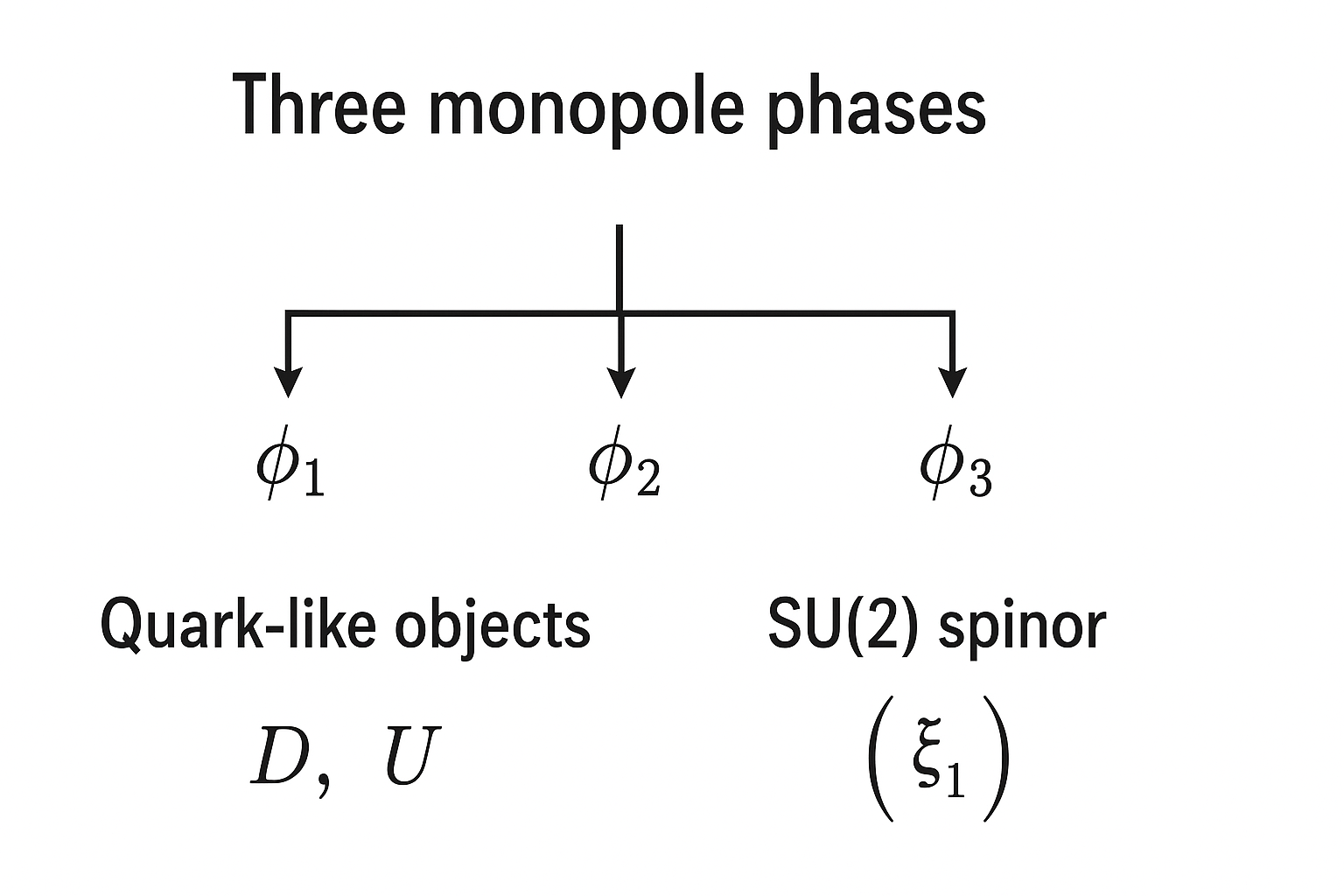
This appendix provides a mathematical justification for the claim: The three monopole phases that determine the quark-like MLTA objects \((D, U)\) are the same three phases that generate the SU(2) spinor, the Hopf soliton, and spin-1/2. No additional internal coordinates, fields, or degrees of freedom are introduced.

We show that: (1) three monopole phases reduce to two independent parameters; (2) the same parameters construct both the quark-like objects and the normalized Hopf spinor; (3) the Hopf curvature produces the invariant \(\psi\); (4) the \(4\pi\) periodicity of the phases enforces spin-1/2; (5) the MLTA unit-number structure forces confinement of \(D\) and \(U\).

Relation to Quantum Field Theory

The framework presented in this work is geometric rather than operator-based, but it is not intended as an alternative to quantum field theory (QFT). Rather, it offers a possible underlying geometric substrate from which key QFT structures may emerge. Several points clarify the relationship.

1. The framework is compatible with QFT's observable content. The construction reproduces the electron's mass, charge, wavelength and spin-1/2 behaviour—the very quantities that QFT attributes to the Dirac field and its gauge interaction with \(U(1)_{\mathrm{em}}\). No prediction contradicts established QED or Standard Model physics. Instead, the MLTA geometry supplies a compact explanation for why the electron field carries these particular quantum numbers.
2. The phases \((\phi_1,\phi_2,\phi_3)\) play the role of internal gauge degrees of freedom. In QFT, an electron field \(\psi(x)\) transforms under local \(U(1)\) phases, and the resulting gauge curvature gives rise to electromagnetism. In the MLTA construction, three monopole phases encode an internal \(U(1)\times U(1)\) structure that—through the holonomy condition—reduces to two independent parameters, matching an SU(2) spinor. Thus the "wave" part of the electron appears as the holonomy of internal geometric directions rather than as a fundamental quantized field. This is conceptually similar to the way spin and isospin arise from internal fibers in geometric quantization and in fiber-bundle formulations of QFT.
3. The Hopf curvature corresponds to the Chern–Simons structure underlying fermion number in QFT. The Chern–Simons 3-form \(a\wedge F\) also appears in QFT in several contexts: topological insulators, theta terms, and anomaly inflow. Here the same mathematical object gives a holonomy measure \(H=\sigma_e^3/(2\pi)\) that reproduces the electron invariant \(\psi\). Thus, the geometric electron can be viewed as a "pre-field" configuration whose curvature resembles the topological sector of the Dirac field. While not strictly quantized, the construction mirrors the field-theoretic interplay between gauge phases, topology, and spin.
4. The quark-like charges arise from MLTA unit-number algebra, not from new quantum fields. Standard QFT introduces independent Dirac fields for \(u\) and \(d\) quarks. The present framework does not posit new fields; rather, it shows that the fractional charges \(-\frac13 e\) and \(+\frac23 e\) appear automatically from the MLTA base-15 structure applied to the same three monopole phases. This suggests that the QFT quark charges may arise as effective representations of deeper geometric relations.
5. The approach can be interpreted as supplying the "initial data" for a QFT description. QFT describes the dynamics of quantized excitations on top of a set of internal symmetries (spin, charge, topology) that are inserted by hand. The MLTA construction proposes that these symmetries—including SU(2) spin, U(1) charge, fractional quark charge, and spin-1/2 double-valuedness—emerge from the topology and holonomy of three underlying monopole phases. In this sense the present framework occupies a level "beneath" the usual QFT description: it sets the geometry that the QFT fields must then respect.
6. Dynamics remain described by QFT. Nothing in this geometric model replaces propagators, interaction terms, or renormalization. These remain part of the conventional QFT description. The MLTA geometry does not supply new scattering amplitudes or modify QED predictions. Instead, it provides a candidate explanation for the origin of the electron's internal quantum numbers and the structure of its wave-state.

In summary: The MLTA geometric framework is best viewed as a geometric pre-structure whose phase holonomy reproduces the quantum numbers that QFT ordinarily takes as axiomatic. Rather than a replacement for quantum field theory, it provides a possible geometric foundation for why the Dirac field has the properties it does.

A.1. Three monopole phases and the holonomy constraint

Let \((\phi_1,\phi_2,\phi_3)\) be the phase directions of the three dimensioned monopole objects \((AL,AL,AL)\) (or \((AL,AV,AV)\) in the positron–proton sector). The cubic holonomy condition,

removes one degree of freedom. Thus: 3 phases → 2 independent parameters, which matches the SU(2) spinor. This means any construction using these phases lies naturally on the two-dimensional manifold underlying the Hopf map \(S^3\to S^2\).

A.2. Removing physical units: from MLTA objects to phases

A dimensioned monopole, such as \(\sigma_e = AL\), \(\sigma_t = AV\), carries MLTA units but appears in the electron only through the dimensionless combination \(\psi = \frac{\sigma_e^3}{2T}\). Because \((u^{-10})^3/(u^{-30}) = 1\), the MLTA magnitudes cancel identically. Therefore the only surviving degree of freedom carried by each monopole is a direction in its internal space, which we write as a unit complex phase: \(\hat{\sigma}_i = e^{i\phi_i}\).

Geometric meaning of "phase" for \(AL\) and \(AV\). A dimensioned monopole object such as \(AL\) or \(AV\) possesses both a physical magnitude (its MLTA dimensional content) and an internal orientation. When these objects enter the electron invariant \(\psi = \frac{\sigma_e^{3}}{2T}\), the MLTA magnitudes cancel exactly: \((u^{-10})^3 / (u^{-30}) = 1\). Thus the only surviving information carried by each monopole is its unit-norm internal direction. A unit direction in an internal \(U(1)\) fiber is naturally represented as a complex phase: \(\hat{\sigma}_i \to e^{i\phi_i}\). In this sense the "phase" of an \(AL\) or \(AV\) object is not its physical size or MLTA content but the dimensionless direction that remains after normalization. These are precisely the degrees of freedom that enter the SU(2) spinor and generate the Hopf curvature. Thus the phases \((\phi_1,\phi_2,\phi_3)\) are the geometric residues of the three MLTA monopoles once all physical units have divided out. The correspondence is: \(AL,\ AV \to e^{i\phi_i}\).

A.3. Construction of the Hopf spinor

The normalized SU(2) spinor is constructed as

The key ansatz,

follows from two natural assumptions: (i) equal per-monopole amplitude (so \(|z_1|^2 \propto 2a^2\), \(|z_2|^2 \propto a^2\), normalization gives \(|z_1|^2=2/3\), \(|z_2|^2=1/3\)); (ii) coherent phase addition (\(e^{i\phi_1}+e^{i\phi_2}\propto e^{i(\phi_1+\phi_2)/2}\)). Thus Eq. (49) is the unique normalized spinor compatible with the symmetry of the three monopoles.

A.4. Hopf curvature and the invariant \(\psi\)

The \(\mathbb{C}P^1\) gauge potential and curvature are \(a_i = -i\xi^\dagger\partial_i\xi\), \(F_{ij} = \partial_i a_j - \partial_j a_i\). The Hopf invariant is

Direct substitution of the ansatz yields

Thus: The same three phases produce the electron's invariant \(\psi\). This establishes the core link: the cubic monopole structure and the Hopf soliton are the same object expressed in MLTA vs SU(2) language.¹

A.5. Spin-1/2 from the phase structure

A \(2\pi\) global phase shift, \(\phi_i \mapsto \phi_i + 2\pi\), gives \((z_1,z_2)\mapsto -(z_1,z_2)\), so the spinor changes sign. Only a \(4\pi\) rotation returns it to itself. Thus: The monopole phase structure transforms exactly like a spin-1/2 object. This requires no new assumptions: the phase structure supplying the quark objects also enforces the SU(2) double-valued representation.

A.6. Relation to the quark-like objects \(D\) and \(U\)

The MLTA unit-number assignments give \(\theta(AL)=-10\), \(\theta(AV)=20\). These correspond to the fractionally charged composites \(D: -\frac13 e\), \(U: +\frac23 e\). Crucially: \(D\) and \(U\) inherit their phase angles from the same \(\phi_i\) that enter the spinor; \(DDD\) and \(DUU\) cancel MLTA scalars, reproducing electrons and positrons; no single \(D\) or \(U\) is dimensionless: the scalar remnants forbid free quarks. Thus: quark-like charges ⇔ monopole phases ⇔ spinor phases.

A.7. The N–S axis and geometric origin of spin-1/2

Article 2 introduced a global geometric "N–S" axis and showed how a particle's discrete tilt with respect to this axis determines its observed 3D motion. Article 4 further developed the N–S axis concept, showing that hypersphere expansion along N–S decomposes into radial and rotational components, creating helical trajectories in 4D that encode quantum numbers (\(n,l,m_l,m_s\)). The present section links that external N–S axis to the internal monopole (DDD) geometry and explains how the three internal phases produce the spin-1/2 transformation law under spatial rotations about the N–S direction.

Physical picture: internal orientation ⇔ N–S axis. Each monopole carries an internal unit direction \(\hat{\sigma}_i=e^{i\phi_i}\) and an associated small internal "N–S" axis (the local internal axis of the monopole phase). When the wave-state is present these internal axes are not spatial vectors but elements of the internal SU(2)/CP\(^1\) bundle. A global spatial rotation about the external N–S axis is represented in the internal bundle by a collective SU(2) rotation of the spinor \(\xi\). Thus the crucial question becomes: how do the three internal monopole directions combine so that a \(2\pi\) spatial rotation yields \(\xi\mapsto -\xi\) (i.e. spin-1/2)?

Two minimal geometric mechanisms:

• (A) Symmetric 120° arrangement (equal-phase, equal-tilt). Place the three monopole internal axes symmetrically around the internal fiber so their azimuthal positions differ by \(2\pi/3\). In Hopf-like constructions such symmetric triads map to a hedgehog-like internal direction field \(\mathbf{n}(x)\) with full SU(2) structure. Under a collective spatial rotation about the external N–S axis the entire spinor undergoes the SU(2) rotation \(U(\hat{n},\theta)=\exp(i\frac{\theta}{2}\,\hat{n}\!\cdot\!\boldsymbol{\sigma})\). For \(\theta=2\pi\) this gives \(U=-\mathbb{I}\) and hence \(\xi\mapsto-\xi\). The symmetric \(2\pi/3\) separation ensures the internal \(\mathbf{n}\) constructed from the three phases follows the spatial rotation coherently, so the collective lift to SU(2) is realized and the system behaves as a spin-1/2 object.
• (B) Tilted-axis cancellation (subtle tilt offsets). Alternatively, each monopole's internal N–S axis may be slightly tilted with respect to the common external axis. If the three tilt vectors are chosen so that their vector sum under a \(2\pi\) spatial rotation returns a collective internal rotation equal to \(2\pi\) in SU(2) (i.e. gives a net factor \(-1\) on \(\xi\)), then again the double-valuedness follows. Concretely, if the internal rotation contributed by monopole \(i\) under a spatial rotation of angle \(\theta\) is \(\delta\varphi_i(\theta)\), we require the collective internal angle \(\Delta\Phi(\theta)=\sum_i \delta\varphi_i(\theta)\) to satisfy \(\Delta\Phi(2\pi)=2\pi\) (so the SU(2) action is \(U(2\pi)=-\mathbb{I}\)). Small, unequal tilt angles thus can add coherently to produce the required half-angle mapping without any monopole individually supplying a half-turn.

A short SU(2) justification. Let \(\xi\) denote the internal two-component spinor constructed from \(\{\phi_i\}\). Spatial rotations about the external N–S axis are represented on fields by the action of the rotation group \(SO(3)\). SU(2) is the double cover of \(SO(3)\); spatial rotation \(R(\theta)\in SO(3)\) lifts to either of two SU(2) elements \(\pm U(\theta)\) where \(U(\theta)=\exp(i\frac{\theta}{2}\,\hat{n}\!\cdot\!\boldsymbol{\sigma})\). If the internal configuration is such that a single spatial rotation by \(\theta=2\pi\) corresponds to the internal action \(U(2\pi)=-\mathbb{I}\) on \(\xi\), then \(\xi\mapsto-\xi\) and the system realizes spin-1/2. This requirement is purely group-theoretic: it only demands the internal collective coordinate (the monopole triad) furnish the fundamental SU(2) representation. The symmetric \(2\pi/3\) arrangement or the tilt-sum arrangement are two geometric ways to guarantee that the internal collective rotation equals the SU(2) half-angle lift of the spatial rotation.

Concrete parametrization (useful for numeric checks). A convenient family interpolating the two mechanisms is obtained by letting each monopole phase depend on the azimuthal coordinate \(\varphi\) and a tilt parameter \(\epsilon_i\): \(\phi_i(\varphi)=\varphi + \psi_i(\epsilon_i)\), \(i=1,2,3\), with \(\psi_i\) encoding local tilt offsets and the cubic constraint \(\sum_i\phi_i=\sigma_e^3\) imposed globally. Under a spatial rotation \(\varphi\mapsto\varphi+\theta\) the spinor phases shift by \(\theta\) plus the tilt contributions. The condition for spin-1/2 is \(\sum_{i=1}^3\big(\Delta\phi_i(2\pi)\big)=2\pi \Rightarrow \xi\mapsto -\xi\). This equality can be checked numerically once a profile for \(\psi_i\) is chosen; it provides a concrete test of whether a chosen monopole geometry yields the desired SU(2) lift.

Remarks on uniqueness and stability. The spin-1/2 outcome is not unique to the symmetric \(2\pi/3\) picture. Any monopole-phase configuration that furnishes the fundamental SU(2) representation under collective rotation will exhibit the same double-valuedness. Energetic or dynamical considerations (soliton profile, minimal energy under the CP\(^1\)/Faddeev-type action) will pick out the physically preferred internal arrangement; symmetric and near-symmetric configurations are typically local minima in standard Hopf-soliton problems. The cubic holonomy \(\psi=\sigma_e^3/(2\pi)\) acts as the global constraint that ties local phase choices together; it ensures the three-phase system cannot be deformed arbitrarily without changing the invariant that determines mass and wavelength.

Summary. The spin-1/2 transformation law is a direct consequence of the collective SU(2) action on the internal monopole triad. Geometrically, this collective action can be realized by a symmetric \(2\pi/3\) phase arrangement or by a coherent sum of small tilts; both mechanisms lift a spatial \(2\pi\) rotation to the SU(2) element \(-\mathbb{I}\) on \(\xi\). Either picture fits naturally into the MLTA/Hopf construction and ties the internal DDD structure to the Article 2 N–S axis.

Cross-reference note: Article 4 provides a complementary "helix-on-helix" perspective on spin-1/2: the electron executes a tight spin helix (scale \(\lambda_e\)) nested inside a larger orbital helix (scale \(n^2 a_0\)). The spin helix completes a half-rotation (\(\pi\) radians) per Compton wavelength, explaining the \(4\pi\) periodicity. Both the present SU(2) phase approach and Article 4's helical trajectory approach describe the same geometric origin of spin-1/2—one from the internal phase structure, the other from the external spacetime path.

A.8. Final synthesis

All of the following emerge from the same three phases obeying the holonomy constraint \(\phi_1+\phi_2+\phi_3 = \sigma_e^3\):

No additional internal fields, no extra degrees of freedom, and no new parameters were introduced. The electron's internal geometry is therefore sufficient to encode both its physical parameters (mass, wavelength, charge, spin) and the quark-like substructure implied by the MLTA unit-number rules. This completes the technical validation of the statement quoted in the main text.