Abstract
Embedded within the mathematical electron formula \(\psi = 4\pi^2q^3\) are geometrical objects with attributes of the Planck units[cite: 14]. The object M = 1 is a unit of mass, T = \(\pi\) a unit of time, P = \(\Omega\) as momentum[cite: 14]. The fine structure constant alpha and \(\Omega\) (formed from pi and e) combine into a geometrical AL = \(q = (2^6 3\pi^2\Omega^5/\alpha)\)[cite: 14]. This \(q\) has the units for a magnetic monopole (ampere-meter) giving the electron a \(q^3\) internal structure that suggests quarks could be related to monopoles[cite: 14]. We expand upon this constructing a quark model entirely from the geometrical objects; Ampere, length L and time T (themselves constructs of \(\alpha, \pi\), e)[cite: 14]. We find solutions with (\(D = AL\), charge \(-\frac{1}{3}e\)) and up (\(U = AV\), charge \(+\frac{2}{3}e\))[cite: 14]. The unit relationship rules between these objects permit a DDD electron but the positron would have to be a DUU, the same configuration as the proton, which could explain the matter-antimatter asymmetry, universe neutrality and why the electron proton charge magnitudes are the same[cite: 14]. We then investigate how a DDD configuration could have a spin-1/2[cite: 14].
The mathematical electron model[cite: 2, 14] represents the electron as a geometrical object described by the formula \(\psi\)[cite: 14]. Although dimensionless, this formula encodes the information required for the physical electron parameters (wavelength, frequency, mass, charge) by embedding within its geometry the MLTA objects—analogues of Planck units for mass (\(m_P\)), length (\(l_p\)), time (\(t_p\)), and charge (\(A\))[cite: 14]. The MLTA objects are themselves constructed from three fundamental numbers: the fine structure constant \(\alpha\), a mathematical constant \(\Omega\), and \(\pi\)[cite: 14].
The electron formula \(\psi\) not only embeds these Planck objects but also dictates their frequency thereby conveying the electron parameters[cite: 14]: \[ \psi = 4\pi^2\left(\frac{2^6 3 \pi^2 \Omega^5}{\alpha}\right)^3 = 0.23895453 \times 10^{23},\quad \text{unit} = 1 \] The electron wavelength and mass can then be given by[cite: 14]: \begin{align*} \lambda_e &= 2\pi l_p \psi \\ m_e &= \frac{m_P}{\psi} \end{align*} Thus, the formula \(\psi\), which resembles the volume of a torus or surface of a 4-D hypersphere, is argued to be a geometrical object that encodes the necessary information required for the physical electron parameters[cite: 14].
(From Article-6: Natural Planck units MTP and the Fine Structure Constant alpha)[cite: 9, 14]. The model uses 3 primary geometrical objects as the Planck units; mass \(M=1\), time \(T=\pi\) and \(P=\Omega\) and in the radiation domain the fine structure constant \(\alpha\)[cite: 14]. Note that \(\Omega\) is a function of the mathematical constants \(\pi\) and Euler's number \(e = 2.718281828459\dots\) (see Article 1b for Omega reference)[cite: 4, 14]: \[ \Omega = \sqrt{\pi^e e^{1-e}} = 2.0071349543\dots \]
As geometrical objects, we can combine MTP to form more complex objects, from electrons to galaxies[cite: 14]. An apple has mass because embedded within the apple are the mass units \(M\)[cite: 14]. However this requires a unit number relationship \(\theta\) that dictates how these objects may combine[cite: 14]. We can assign to the \(\mathrm{kg}\); \(\theta = 15\), to \(\mathrm{s}\), \(\theta = -30\), ... from these and from the base-15 rule set that governs these relationships we can build Table 1[cite: 14].
Each object is assigned a dimensioned scalar (these combine a numerical value with a dimensioned unit)[cite: 14]. For example we may assign \(M=(1)k = m_P\), \(T=(\pi)t = t_p\), \(V=(2 \pi \Omega^2)v = c\)...[cite: 14] The number ruling \(\theta\) applies to the scalars and so we find that only two scalars are required to be assigned values (numerical and units), this is because the base-15 rule set constraints force all others — the system is exactly determined[cite: 14]. In this model the two scalars chosen are \(r\) (\(\theta = 8\)) and \(v\) (\(\theta = 17\)) as \(v = c/(2 \pi \Omega^2)\) (and so has an exact solution) and \(r\) has only integer exponents[cite: 14]. In SI units: \[ v,\text{units} = \frac{\mathrm{m}}{\mathrm{s}}, \qquad r, \text{units} = \left(\frac{\mathrm{kg} \cdot \mathrm{m}}{\mathrm{s}}\right)^{1/4} \]
| Attribute | Quantity | Object | Scalar | \(u^{\theta}\) | unit |
|---|---|---|---|---|---|
| mass | \(M\) | \((1)\) | \(\dfrac{r^{4}}{v}\) | \(u^{15}\) | kg |
| time | \(T\) | \((\pi)\) | \(\dfrac{r^{9}}{v^{6}}\) | \(u^{-30}\) | s |
| sqrt momentum | \(P\) | \(\Omega M^{(4/5)} {\left(\dfrac{\pi}{T}\right)}^{(2/15)} = (\Omega)\) | \(r^{2}\) | \(u^{16}\) | \(\sqrt{\dfrac{\mathrm{kg\,m}}{\mathrm{s}}}\) |
| velocity | \(V\) | \(\dfrac{2\pi P^{2}}{M}=(2\pi\Omega^{2})\) | \(v\) | \(u^{17}\) | m/s |
| length | \(L\) | \(VT=(2\pi^{2}\Omega^{2})\) | \(\dfrac{r^{9}}{v^{5}}\) | \(u^{-13}\) | m |
| current | \(A\) | \(\dfrac{2^{4}V^{3}\alpha}{P^{3}}=(2^{7}\pi^{3}\alpha \Omega^{3})\) | \(\dfrac{v^{3}}{r^{6}}\) | \(u^{3}\) | A |
| temperature | \(K\) | \(\dfrac{AV}{2\pi}=(2^{7}\pi^{3}\alpha\Omega^{5})\) | \(\dfrac{v^{4}}{r^{6}}\) | \(u^{20}\) | K |
The mathematical electron formula \(\psi\) incorporates dimensioned Planck units but is itself dimensionless (units = scalars = 1)[cite: 14]. \[ \psi = 4\pi^2 (2^6 3 \pi^2 \alpha^{-1} \Omega^5)^3 = 2^{20} \pi^8 3^3 \alpha^{-3} \Omega^{15} = 0.23895453\dots \times 10^{23} \] Nevertheless \(\psi\) contains the information needed to reproduce all physical electron parameters[cite: 14]. Here we summarise the result in a compact form, since it underlies all later sections of this article[cite: 14]. From Table 1[cite: 14].
Time: \[ T = \pi \frac{r^9}{v^6},\quad u^{-30} \] \(AL\) (the units for the magnetic monopole are the ampere-meter)[cite: 14]: \begin{align*} \sigma_e &= \frac{3 \alpha^{-2} A L}{2\pi^2} = 2^7 3 \pi^3 \alpha^{-1} \Omega^5,\quad \text{unit} = u^{-10},\quad \text{scalars} = \frac{r^3}{v^2} \\ \psi &= \frac{\sigma_e^3}{2 T} = \frac{(2^7 3 \pi^3 \alpha^{-1} \Omega^5)^3}{2\pi},\quad \text{unit} = \frac{(u^{-10})^3}{u^{-30}}=1,\quad \text{scalars} = \left(\frac{r^3}{v^2}\right)^3 \frac{v^6}{r^9}=1 \\ \psi &= 2^{20} \pi^8 3^3 \alpha^{-3} \Omega^{15},\quad \text{unit} = 1,\quad \text{scalars} = 1 \end{align*}
1. Mass
The electron mass is the Planck mass scaled by the inverse winding number[cite: 14]:
\[
m_e = \frac{m_P}{\psi}.
\]
2. Wavelength
The Compton wavelength is the Planck length scaled by the same winding number[cite: 14]:
\[
\lambda_e = 2\pi l_P\, \psi.
\]
3. Frequency
The internal oscillation frequency is the winding number measured in Planck time units[cite: 14]:
\[
\nu_e = \frac{\psi}{t_P}.
\]
4. Charge
Because the electric charge arises from the embedded monopole geometry \(A\,T\), the elementary charge satisfies[cite: 14]
\[
e = A T,
\]
with \(A\) and \(T\) already fixed by \(\alpha\) and \(\Omega\)[cite: 14].
Thus all observable electron parameters \((m_e,\ \lambda_e,\ \nu_e,\ e)\) follow directly from the single invariant[cite: 14] \[ \psi=\frac{\sigma_e^3}{2\pi}, \] which is the cubic monopole holonomy of the wave-state[cite: 14]. Nothing beyond the MLTA geometrical objects \((M,L,T,A,V)\) and the constants \((\alpha,\Omega,\pi)\) is required, and these are all embedded within the formula for \(\psi\)[cite: 14].
Particle mass is a unit of Planck mass that occurs once per \(\psi\) units of Planck time, while other parameters are continuums of Planck units[cite: 14]: \[ m_e = \frac{m_P}{\psi}, \] The electron is modelled not as a physical entity but rather as an oscillation between 2 distinct states; an electric wave-state (duration particle frequency) and a mass point-state (duration 1 unit of Planck time)[cite: 14]. At a given Planck time unit the electron occupies a point (mass) state of duration one Planck time \(t_P\)[cite: 14]. In this state the electron is dimensionless: the algebraic units in the formula (the \(\mathrm{AL}^3/T\) factors) cancel and no electric wave-state substructure is present[cite: 14]. The point state therefore functions as a marker in the Planck-unit scaffolding of the universe rather than as a classical extended object[cite: 14]. The model identifies the electron mass with a Planck mass rescaling[cite: 14]. Immediately following the point state, the electron unfolds into a wave (phase) state of duration[cite: 14] \[ T_{\mathrm{wave}} = \psi\, t_P. \] During the wave state there is no intrinsic mass density: the physical degrees of freedom are purely topological phase units (the monopole amplitudes \(\sigma_e\)) whose non-abelian holonomy realizes \(\psi=\sigma_e^3/(2\pi)\)[cite: 14].
Mass as average mass. Electron mass is a unit of Planck mass that occurs only once per \(\psi\) units of Planck time, the other parameters are continuums of the Planck units[cite: 14].
This may be interpreted as; for \(\psi\) units of Planck time the electron has wavelength L, charge A ... and then the AL combine with time T (\(A^3L^3/T\)) and the units (and scalars) cancel[cite: 14]. The electron is now mass (for 1 unit of Planck time)[cite: 14]. In this consideration, the electron is an event that oscillates over time[cite: 14]. Thus the electron is a quantum scale event, it does not exist at the discrete Planck scale (and so therefore neither does the quantum scale)[cite: 14].
As electron mass is the frequency of the geometrical Planck mass M = 1, which is a point (and so with point co-ordinates), then we have a model for a black-hole electron, the electron function \(\psi\) centered around this unit of Planck mass (see spiral Article 1b)[cite: 4, 14]. When the wave-state units collapse, this black-hole center (point) is defined for 1 unit of (Planck) time[cite: 14]. The electron is 'now' (a unit of Planck) mass[cite: 14].
Mass in this consideration is therefore not a constant property of the particle, rather the measured particle mass \(m\) would refer to the average mass, the average occurrence of the discrete Planck mass point-state over time[cite: 14]. The formula \(E = hf\) is a measure of the frequency \(f\) of occurrence of Planck's constant (a fixed constant) and applies to the electric wave-state[cite: 14]. As for each wave-state there is a corresponding mass point-state, then for a particle \(hf == mc^2\)[cite: 14]. Notably however the \(c\) term is the fixed constant unlike the \(f\) term, and so the \(m\) term is the frequency term, it is referring to an average mass (mass which is measured over time) rather than a constant mass (mass as a constant property of the particle at unit Planck time)[cite: 14]. Thus when we refer to mass as a constant property, we are actually referring to mass reading at the quantum scale[cite: 14].
The \(\tau\)-loop wave-state engine. When this article was originally drafted, the exact mathematical mechanism for the wave-state was unknown[cite: 14]. With the derivation of the \(\tau\)-loop continuous evaluation engine (Article 1b)[cite: 4, 14], we now know that this "unfolding" corresponds to the continuous evaluation of the wave-state amplitude \(A(\tau) = \Omega^{\ln\tau+1}\) as the simulation sweeps through the internal interval \(\tau \in [1,e]\)[cite: 14]. The electron's wavelength, spin and topological current are properties of this continuous phase trajectory[cite: 14]. Mass reappears only when the \(\tau\)-loop reaches its natural boundary at \(\tau=e\), triggering Euler's identity (\(e^{i\pi}=-1\)) and forcing the complex wave-state to collapse back to the real coordinate axis for the next Planck tick point state[cite: 14].
The charge on the electron derives from the embedded ampere \(A\) and length \(L\), while the electron formula \(\psi\) itself is dimensionless[cite: 14]. These AL have the units for magnetic monopoles (ampere-meter) and appear analogous to quarks (3 monopoles per electron), but the perfect symmetry and stability of \(\psi\) provide no clear fracture point for electron disruption and so any internal electron structure would be from difficult to impossible to detect/measure[cite: 14]. AL magnetic monopoles: \begin{align*} \sigma_e &= \frac{3 \alpha^{-2} A L}{2\pi^2} = 2^7 3 \pi^3 \alpha^{-1} \Omega^5,\quad \text{unit} = u^{-10},\quad \text{scalars} = \frac{r^3}{v^2} \\ \psi &= \frac{(2^7 3 \pi^3 \alpha^{-1} \Omega^5)^3}{2\pi},\quad \text{unit} = \frac{(u^{-10})^3}{u^{-30}}=1,\quad \text{scalars} = \left(\frac{r^3}{v^2}\right)^3 \frac{v^6}{r^9}=1 \end{align*}
If the magnetic monopole \(\sigma_e\) could equate to a quark with electric charge \(-\frac{1}{3}e\), it would be an analogue of the D quark[cite: 14]. Three D quarks would constitute the electron as DDD = (AL)\(\times\)(AL)\(\times\)(AL)[cite: 14].
For the positron (anti-matter electron), we might expect the inverse charge, but AL units \(\theta = -10\), and no 'units \(\theta = +10\)' combination including A exists in the set of unit number relations[cite: 14]. However, we can also derive our electron formula via a Planck temperature \(t_p\) AV monopole (ampere-velocity)[cite: 14]: \begin{align*} t_p &= 2^7 \pi^3 \alpha \Omega^5,\quad \text{units} = u^{20},\quad \text{scalars} = \frac{r^9}{v^6} \\ \sigma_t &= \frac{3 \alpha^{-2} t_p}{2\pi} = \frac{3 \alpha^{-2} A V}{2\pi^2} = (2^6 3 \pi^2 \alpha^{-1} \Omega^5),\quad \text{units} = u^{20},\quad \text{scalars} = \frac{v^4}{r^6} \\ \psi &= {(2T)}^2 \sigma_t^2 \sigma_e = 2^{20} 3^3 \pi^8 \alpha^{-3} \Omega^{15},\quad \text{unit} = (u^{-30}) (u^{20})^2 (u^{-10}) = 1, \quad \text{scalars} = 1 \end{align*}
The units for \(\sigma_t\) unit number \(\theta = +20\), so if \(\theta = -10\) equates to \(-\frac{1}{3}e\), then \(\theta = +20\) may equate to \(+\frac{2}{3}e\), analogous to the U quark, the difference between them being a unit of time T (\(\theta = -30\))[cite: 14]. The positron charge structure becomes DUU, resembling the proton's quark structure rather than simply being the electron's inverse[cite: 14]. This could explain missing anti-matter and why proton and electron charge magnitudes match exactly[cite: 14]. \begin{align*} D &= \sigma_e,\quad \text{unit} = u^{-10},\quad \text{charge} = -\frac{e}{3},\quad \text{scalars} = \frac{r^3}{v^2} \\ U &= \sigma_t,\quad \text{unit} = u^{20},\quad \text{charge} = \frac{2e}{3},\quad \text{scalars} = \frac{v^4}{r^6} \end{align*}
Numerically: Adding proton (UUD) and electron (DDD) gives 2(UDD) = 20 - 10 - 10 = 0 (zero charge), scalars = 0[cite: 14]. Converting between U and D via U & DDD (electron) = 20 - 10 - 10 - 10 = -10 (D), scalars = \(\dfrac{r^3}{v^2}\)[cite: 14]. The quark/monopoles themselves have physical units (the scalars have not cancelled) but experimental physics suggests that these combinations are unstable independent of other quarks[cite: 14].
Both DDD and DUU variations yield the same electron geometry and so in this respect the electron and positron are the same[cite: 14]; \[ \psi = \frac{\sigma_e^3}{2 T} = 2^{20} 3^3 \pi^8 \alpha^{-3} \Omega^{15} \] \[ \psi = {(2T)}^2 \sigma_t^2 \sigma_e = 2^{20} 3^3 \pi^8 \alpha^{-3} \Omega^{15} \]
| Combination | \(\theta\) | Interpretation |
|---|---|---|
| \(AL\) | \(3 + (-13) = -10\) | Down quark: \(-\frac{1}{3}e\) |
| \(AV\) | \(3 + 17 = 20\) | Up quark: \(+\frac{2}{3}e\) |
| \(AT\) | \(3 + (-30) = -27\) | Electron charge: \(-e\) |
Observation: Positron and proton have identical \(\theta = +30\) and charge \(+e\), however the positron has independent quarks whereas the proton has complex quarks (the 1836 \(\times\) mass difference)[cite: 14]. From this we may premise that the electron and positron quarks are free (with minimum binding), but the proton and neutron quarks are significantly constrained (a complex internal structure)[cite: 14]. We cannot therefore directly compare these quarks as discrete units, but we can reference both sets[cite: 14].
A key design goal of the MLTA framework is low descriptive complexity: new phenomena should be representable using the same small set of primitives \((\alpha,\Omega,\pi)\) and the same MLTA objects that already generate the electron invariant \(\psi\)[cite: 14]. Since we showed that the electron embeds quark-like monopole objects \(D=AL\) and \(U=AV\), the natural next question is whether the photon can be represented by a closely related internal structure, so that “the easiest thing to mix with water is more water”: particles and photons would then share a common geometric substrate[cite: 14].
Monopole blocks carry the same \(\Omega^5\) geometry.
From the MLTA definitions[cite: 14],
\[
L\propto \Omega^{2},\qquad V\propto \Omega^{2},\qquad A\propto \Omega^{3},
\]
so the two quark-like monopole blocks
\[
D\equiv AL,\qquad U\equiv AV
\]
share the same underlying \(\Omega\)-power[cite: 14]:
\[
AL\propto \Omega^{2}\Omega^{3}=\Omega^{5},\qquad
AV\propto \Omega^{2}\Omega^{3}=\Omega^{5}.
\]
Thus Article 5's \(Q^{2}Q^{3}=Q^{5}\) structure acquires physical dimensionality here: it is precisely the monopole/quark building rule[cite: 8, 14].
A neutral, scalar-free triplet exists: \(\gamma \equiv DDU\).
Consider the composite[cite: 14]
\[
\gamma \;\equiv\; DDU \;=\; (AL)^2(AV).
\]
Using the unit numbers \(\theta(AL)=-10\) and \(\theta(AV)=+20\)[cite: 14],
\[
\theta(\gamma)=2(-10)+20=0,
\]
so \(\gamma\) is dimensionless in the MLTA unit-number algebra[cite: 14]. It is also scalar-free[cite: 14]. From the scalar content already derived[cite: 14],
\[
D:\ \frac{r^3}{v^2},\qquad U:\ \frac{v^4}{r^6},
\]
so
\[
\text{scalars}(\gamma)=
\left(\frac{r^3}{v^2}\right)^2\left(\frac{v^4}{r^6}\right)=1.
\]
Therefore \(\gamma\) is a purely geometric object: units \(=1\) and scalars \(=1\)[cite: 14].
Finally, the \(\Omega\)-power of \(\gamma\) is[cite: 14] \[ \gamma \;\propto\; (\Omega^{5})^3=\Omega^{15}. \] This links the photon candidate directly to the base-15 residue already identified as fundamental in the dimensionless sector[cite: 14]. As proven analytically in Article 1b, \(\Omega^{15}\) is precisely the "master scalar" \(i\)—the unique minimal positive solution to the lattice Diophantine condition that allows the \(\tau\)-loop phase cycles to close synchronously[cite: 4, 14]. The photon primitive \(\gamma\propto\Omega^{15}\) is therefore a perfect geometric fit for the 15-tick dimensional closure of the simulation lattice[cite: 14].
Charge neutrality.
If \(D\) and \(U\) are interpreted as carrying \(-\tfrac13 e\) and \(+\tfrac23 e\) respectively (as derived from the MLTA rule set)[cite: 14], then
\[
q_\gamma \;=\; 2\!\left(-\tfrac13 e\right) + \left(+\tfrac23 e\right)=0,
\]
so \(\gamma\) is electrically neutral, consistent with the photon[cite: 14].
Within the MLTA bookkeeping, the electron and positron are built from the same monopole blocks but differ in how the unit-number constraints permit charge reversal[cite: 14]: \[ e^- \sim DDD,\qquad e^+ \sim DUU. \] A six-block \(e^-e^+\) system can be repartitioned without introducing any new primitives[cite: 14]: \[ DDD + DUU \;\;\longrightarrow\;\; (DDU) + (DDU) \;\;\equiv\;\; \gamma + \gamma. \] This is not proposed as a replacement for QED, but as a geometric reinterpretation of the observed two-photon final state: “annihilation” is expressed here as a recombination of internal MLTA monopole blocks into two neutral, scalar-free, \(\Omega^{15}\) composites[cite: 14].
Why two photons and opposite directions.
The repartitioning naturally produces two neutral composites[cite: 14]. Momentum conservation then requires the two resulting photons to carry equal and opposite momenta in the center-of-mass frame[cite: 14]. In the present geometric language this can be represented as opposite orientations of the same dimensionless \(\Omega^{15}\) residue (a \(+\) and a \(-\) configuration), yielding two counter-propagating photon states[cite: 14].
Energy and frequency remain conventional.
Although \(\gamma\) is dimensionless (units = scalars = 1), observable photon frequency is fixed by the usual energy balance[cite: 14]. In the rest frame of the initial \(e^-e^+\) pair[cite: 14],
\[
E_{\gamma 1}=E_{\gamma 2}=m_e c^2,\qquad \nu_\gamma=\frac{E_\gamma}{h}=\frac{m_e c^2}{h}.
\]
Since \((m_e,c,h)\) are already generated within the MLTA framework from the same underlying constants and scalars, the photon frequency introduces no new degrees of freedom[cite: 14].
Kolmogorov/MDL interpretation.
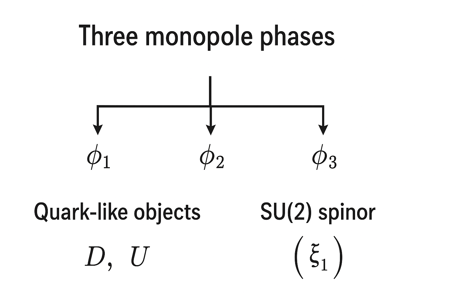
The significance of this construction is compression: the photon analogue \(\gamma\) requires no new constants, no new unit-number rules, and no extra internal coordinates beyond the three monopole phases used for the electron invariant \(\psi\)[cite: 14]. Thus the conceptual cost of adding photons to the model is minimal: particles and photons are built from the same \(\Omega^5\) blocks, and their composites differ primarily by how the unit-number constraints allow neutral, scalar-free cancellations[cite: 14]. In MDL terms, the model reuses the same short “program” to generate both charged fermionic structure and neutral radiative structure[cite: 14].
The purpose of this quark construction is to show that the MLTA geometric rules—the same rules that generate the electron—also support a natural analogue of quark structure[cite: 14]. Several features make this plausible[cite: 14]:
1. Quark charges emerge without input.
The unit-number rule (base-15 geometry) assigns[cite: 14]
\[
\theta(AL)=-10,\qquad \theta(AV)=+20,
\]
and these correspond exactly to the fractional charges[cite: 14]
\[
D:\ -\tfrac{1}{3}e,\qquad U:\ +\tfrac{2}{3}e.
\]
No charge values were inserted by hand; they arise from the MLTA geometry alone[cite: 14].
2. Electron–positron asymmetry follows from MLTA constraints.
The electron is \((AL)^3/T\) whereas no \(+10\) unit-number combination exists involving \(A\)[cite: 14]. Therefore the positron cannot be formed from “anti-\(AL\)’’ units; instead it is naturally the \(DUU\) combination[cite: 14]. This offers a geometric explanation for the observed matter–antimatter asymmetry and for why proton and electron charges have the same magnitude[cite: 14].
3. Proton and positron equivalence appears automatically.
The positron is restricted to a DUU configuration[cite: 14].
\[
\theta_{e^+} = -10 + 2(20) = +30,
\]
The proton and positron share the same quark configuration[cite: 14]. This is not an imposed symmetry but an automatic consequence of the geometric rules[cite: 14].
4. Free quarks are forbidden by scalar non-cancellation.
The MLTA scalars do not cancel for individual \(D\) or \(U\) objects[cite: 14]:
\[
D:\ \frac{r^3}{v^2},\qquad U:\ \frac{v^4}{r^6}.
\]
Only triplets (DDD, DUU, UDD) have the necessary combinations that are able to cancel the scalars and yield dimensionless composites[cite: 14]. Thus the model naturally reproduces a confinement-like rule: isolated quark objects cannot exist as stable physical entities[cite: 14].
5. Compatibility with the spin construction.
The same three phases that carry the charge structure and, through the \(\tau\)-loop, spin-1/2[cite: 14]. Thus the charge structure and the spin-\(\tfrac12\) structure arise from the same internal geometry, giving internal consistency with no additional degrees of freedom[cite: 14].
6. No new physical constants.
The entire quark structure derives from \((\alpha,\Omega,\pi) == (\alpha,\pi, e)\) and the base-15 relationship between MLTA objects[cite: 14]. The model introduces no free parameters, matching the philosophy of the mathematical electron[cite: 14].
Taken together, these features make the monopole-based quark model a natural extension of the electron's internal geometry[cite: 14]. It is not offered as a replacement for the QCD quark model, this is a formal analogy rather than a rigorous derivation, but it serves as a demonstration that the same quantity \(\psi\) that encodes the electron also supports a compact and self-consistent quark interpretation (see Appendix for mathematical treatment)[cite: 14].
This appendix examines the claim that the three monopole phases which determine the quark-like MLTA objects \((D,U)\) also carry the electron's spin and charge structure, with no additional internal coordinates, fields or degrees of freedom[cite: 14]. It was first written before the \(\tau\)-loop architecture of Article 1b[cite: 4, 14] had been determined[cite: 14]. It has been revised against that architecture, and corrected where earlier arguments did not survive checking[cite: 14].
The results established are[cite: 14]:
The framework presented here is geometric rather than operator-based, and is not intended as an alternative to quantum field theory (QFT)[cite: 14]. It offers a possible geometric substrate from which some QFT structures may emerge[cite: 14].
(1) Compatibility with QFT's observable content.
The construction reproduces the electron's mass, charge, wavelength and spin-\(\tfrac12\) behaviour — the quantities QFT attributes to the Dirac field and its \(U(1)_{\mathrm{em}}\) interaction[cite: 14]. No prediction contradicts established QED[cite: 14]. The MLTA geometry offers a candidate explanation for why the electron carries these quantum numbers[cite: 14].
(2) The phases as internal degrees of freedom.
In QFT an electron field transforms under local \(U(1)\) phases[cite: 14]. Here three monopole phases, reduced by a holonomy condition, carry two dynamical degrees of freedom[cite: 14]. Whether these furnish the full SU(2) structure of a spinor is a separate question, answered in the negative for the construction of A.3; spin-\(\tfrac12\) is instead obtained topologically in A.5[cite: 14].
(3) Quark-like charges from unit-number algebra, not new fields.
Standard QFT introduces independent Dirac fields for \(u\) and \(d\)[cite: 14]. The present framework posits none: the fractional charges \(-\tfrac13 e\) and \(+\tfrac23 e\) follow from the MLTA base-15 structure, and their confinement from the scalar algebra of A.6[cite: 14].
(4) A candidate source of QFT's initial data.
QFT describes dynamics on top of internal symmetries — spin, charge — that are inserted by hand[cite: 14]. The MLTA construction proposes that these emerge from the \(\tau\)-loop and the unit-number structure, so that the framework sits “beneath” the usual QFT description and fixes the geometry the fields must respect[cite: 14].
(5) Dynamics remain described by QFT.
Nothing here replaces propagators, interaction terms or renormalization[cite: 14]. The geometry supplies no new scattering amplitudes and does not modify QED predictions[cite: 14]. It addresses the origin of the electron's internal quantum numbers, not their dynamics[cite: 14].
In summary: the MLTA framework is best read as a geometric pre-structure whose \(\tau\)-loop and unit-number algebra reproduce quantum numbers that QFT takes as axiomatic[cite: 14].
Let \((\phi_1,\phi_2,\phi_3)\) be the phase directions of the three dimensioned monopole objects \((AL,AL,AL)\), or \((AL,AV,AV)\) in the positron sector[cite: 14]. They are subject to the holonomy condition[cite: 14] \[ \phi_1 + \phi_2 + \phi_3 \equiv \sigma_e^{3} \pmod{2\pi}, \] where \(\sigma_e^{3}\) denotes the scalar-free numerical value[cite: 14]. Since \(\psi = \sigma_e^{3}/2T\) and the object value of \(T\) is \(\pi\)[cite: 14], \[ \sigma_e^{3} \bmod 2\pi = 2\pi\,\bigl(\psi \bmod 1\bigr). \] The holonomy target is therefore not automatically zero[cite: 14]. With the CODATA value of \(\alpha\), \(\psi\) has fractional part \(0.356\) and the target is \(2.238\) rad[cite: 14]. It vanishes only when \(\psi\) is an integer — the synchronisation condition of Article 1b, under which a closure must coincide with a spiral tick[cite: 4, 14]. With integer \(\psi\) the condition becomes \(\sum\phi_j \equiv 0 \pmod{2\pi}\), which, with \(\phi_j = \pi n_j\) at closure, is the Article 1b requirement that the turn numbers satisfy \(\sum n_j\) even[cite: 4, 14].
The constraint removes one degree of freedom[cite: 14]: \[ \underbrace{3 \text{ phases}}_{\phi_1,\phi_2,\phi_3} \;\longrightarrow\; \underbrace{2 \text{ dynamical degrees of freedom}}. \] That two remain is a statement about the phases[cite: 14]. How many of them are visible in a constructed state depends on the construction, and is taken up in A.3[cite: 14].
A dimensioned monopole such as \(\sigma_e = AL\) or \(\sigma_t = AV\) enters the electron only through the dimensionless combination[cite: 14] \[ \psi = \frac{\sigma_e^{3}}{2T}, \] in which both the unit numbers and the translation scalars cancel identically[cite: 14]: \[ \frac{(u^{-10})^{3}}{u^{-30}} = 1, \qquad \frac{(r^{3}v^{-2})^{3}}{r^{9}v^{-6}} = 1. \] The only surviving information carried by each monopole is therefore its unit-norm internal direction, represented as a complex phase[cite: 14]: \[ \hat{\sigma}_i = e^{i\phi_i}. \] The “phase” of an \(AL\) or \(AV\) object is not its physical size or MLTA content, but the dimensionless direction that remains once all units have divided out[cite: 14].
Earlier versions proposed the normalized two-component construction[cite: 14] \[ z_1 = \sqrt{\tfrac{2}{3}}\,e^{i(\phi_1+\phi_2)/2},\qquad z_2 = \sqrt{\tfrac{1}{3}}\,e^{i\phi_3}, \] justified by two assumptions: (i) each monopole contributes equal amplitude \(a\), so \(|z_1|^{2}\propto 2a^{2}\) and \(|z_2|^{2}\propto a^{2}\); and (ii) two phases combining in one amplitude give the average phase \((\phi_1+\phi_2)/2\)[cite: 14].
The two assumptions are mutually inconsistent.
Assumption (i) adds the monopoles' intensities; assumption (ii) adds their amplitudes[cite: 14]. Coherent addition gives the full identity[cite: 14]
\[
e^{i\phi_1} + e^{i\phi_2} = 2\cos\!\Bigl(\tfrac{\phi_1-\phi_2}{2}\Bigr)\, e^{i(\phi_1+\phi_2)/2},
\]
so that \(|z_1|^{2} = 4a^{2}\cos^{2}\bigl((\phi_1-\phi_2)/2\bigr)\), which equals \(2a^{2}\) only when \(\phi_1-\phi_2 = \pm\pi/2\)[cite: 14]. The equation takes its phase from coherent addition and its magnitude from incoherent addition[cite: 14].
Consequence: one visible degree of freedom, not two.
Because \(|z_1|\) and \(|z_2|\) are fixed, the Bloch coordinate \(n_z = |z_1|^{2} - |z_2|^{2} = \tfrac13\) is the same for every choice of phases, and the combination \(\phi_1 - \phi_2\) does not appear at all[cite: 14]. The equation therefore places the state on a single latitude circle of the Bloch sphere[cite: 14]. It carries one state-visible parameter, where a general SU(2) spinor requires two, and the second dynamical degree of freedom of A.1 is real but invisible to it[cite: 14].
A consistent alternative.
Treating the addition coherently throughout, \(z_1 = a(e^{i\phi_1}+e^{i\phi_2})\) and \(z_2 = a\,e^{i\phi_3}\), restores the second parameter: \(n_z = (4\cos^{2}\tfrac{D}{2} - 1)/(4\cos^{2}\tfrac{D}{2} + 1)\) with \(D = \phi_1-\phi_2\), and the relative phase depends on \(\phi_1+\phi_2\)[cite: 14]. This form reaches \(n_z \in [-1, \tfrac35]\) — most of the sphere, but not a polar cap[cite: 14]. It is better, not complete[cite: 14].
Status.
Neither construction delivers a full SU(2) spinor from the phases alone, and the earlier claim that the equation is “the unique normalized spinor” is withdrawn[cite: 14]. Nothing below depends on it: spin-\(\tfrac12\) is established in A.5 by an argument that does not use the ansatz[cite: 14].
Earlier versions of this appendix sought \(\psi\) as the value of a Hopf invariant computed from the spinor ansatz[cite: 14]. That derivation is withdrawn: the Hopf integral requires a spatially varying field, none was specified, and constant phases give zero curvature[cite: 14]. The \(\tau\)-loop architecture of Article 1b[cite: 4, 14] supplies \(\psi\) with a direct meaning instead[cite: 14].
In that architecture every object is a \(\tau\)-loop: an evaluation over \(u = \ln\tau \in [0,1]\) whose amplitude runs from \(\Omega\) to \(\Omega^{2}\) and whose phase advances by \(\pi\) before closure[cite: 14]. The Planck scaffolding completes such a loop at every tick[cite: 14]. The electron is the same loop executed \(\psi\) times more slowly[cite: 14]: \[ \psi = \text{number of Planck ticks in one electron } \tau\text{-loop} = \frac{\sigma_e^{3}}{2T} = 2^{20}\,3^{3}\,\pi^{8}\,\alpha^{-3}\,\Omega^{15} \approx 2.389545\times10^{22}. \]
This fixes the electron's observables without further assumption[cite: 14]. Its time-averaged mass is the slowdown ratio[cite: 14], \[ m_e = \frac{m_P}{\psi}, \] and its loop period is the reduced Compton time, \(\psi\,t_P = \bar\lambda_e/c\), so that \(\bar\lambda_e = \psi\,\ell_P\) and \(\lambda_e = 2\pi\,\psi\,\ell_P\)[cite: 14]. The electron marks the spiral once per loop and deposits nothing further: the ratio \(m_P/\psi\) is a duty cycle, not a quantity of mass laid down[cite: 14]. The distinction between \(\psi\) as a radius-like count and \(\sigma_e^{3} = 2\pi\psi\) as its circumference-like counterpart is the same \(2\pi\) that relates the reduced and full Compton wavelengths[cite: 14].
The \(\tau\)-loop half-cycle.
Each loop advances the phase by[cite: 14]
\[
\varphi_{\text{loop}} = \pi\ln e = \pi,
\]
not \(2\pi\), and closes on \(\Psi(e) = \Omega^{2}e^{i\pi} = -\Omega^{2}\)[cite: 14]. One loop multiplies the state by \(e^{i\pi} = -1\); a second restores it[cite: 14]. If one \(\tau\)-loop corresponds to one complete rotation, then a rotation through \(\theta\) contributes phase \(\theta/2\), which is precisely the half-angle factor \(e^{i\theta/2}\) of a spin-\(\tfrac12\) object[cite: 14]:
\[
\theta = 2\pi \;\longrightarrow\; e^{i\pi} = -1, \qquad \theta = 4\pi \;\longrightarrow\; e^{i2\pi} = +1.
\]
Article 4[cite: 7, 14] reached the same conclusion from the external side, as a spin helix completing half a rotation per Compton wavelength[cite: 14]. That is the same half-cycle, seen as a trajectory rather than as a phase[cite: 14].
The configuration space.
A state that returns after \(4\pi\) but not after \(2\pi\) requires a configuration space in which a \(4\pi\) loop closes and a \(2\pi\) loop does not[cite: 14]. The 3-sphere \(S^{3}\cong \mathrm{SU}(2)\) is that space: it double-covers the rotation group \(\mathrm{SO}(3)\cong\mathbb{RP}^{3}\), so a \(2\pi\) rotation, which is a closed loop in \(\mathrm{SO}(3)\), lifts to a path from a point \(x\) to its antipode \(-x\) on \(S^{3}\), closing only at \(4\pi\)[cite: 14]. The observable orientation is a vector and is \(2\pi\)-periodic; the underlying state lives on \(S^{3}\) and is \(4\pi\)-periodic[cite: 14]. No half-angle is assumed, and no coupling postulate is required: the half-cycle of the \(\tau\) loop and the double cover of \(\mathrm{SO}(3)\) are the same factor of two[cite: 14].
What is and is not claimed.
This shows that spin-\(\tfrac12\) is available to the electron's \(\tau\)-loop, and that its double-valuedness follows from the half-cycle[cite: 14]. It does not by itself explain why some objects realise spin-\(\tfrac12\) and others do not; that selection is left open[cite: 14].
The unit-number assignments are[cite: 14] \[ \theta(AL) = -10,\qquad \theta(AV) = +20, \] corresponding to the fractionally charged objects[cite: 14] \[ D:\ -\tfrac13 e,\qquad U:\ +\tfrac23 e, \] with translation scalars \(D \sim r^{3}v^{-2}\) and \(U \sim r^{-6}v^{4}\)[cite: 14].
Each object's scalars are its charge times \(T\).
Writing \(T \sim r^{9}v^{-6}\), both objects satisfy exactly[cite: 14]
\[
\text{scalars}(q) = -\,Q(q)\times T,
\]
since \(-(-\tfrac13)(9,-6) = (3,-2)\) and \(-(\tfrac23)(9,-6) = (-6,4)\)[cite: 14]. Scalars add under composition, as do charges, so for any composite of total charge \(Q\) the total scalar content is \(-Q\times T\)[cite: 14]. The composite is scalar-free — and so describes an observable object — precisely when multiplied by \(T^{Q}\)[cite: 14].
The power of \(T\) is the charge.
| composite | charge | power of \(T\) | status |
|---|---|---|---|
| \(D,\ U,\ DD,\ DU,\ UU\) | fractional | fractional | confined |
| \(DDD\) | \(-1\) | \(-1\) | electron |
| \(DDU\) | \(0\) | \(0\) | photon |
| \(DUU\) | \(+1\) | \(+1\) | positron |
| \(UUU\) | \(+2\) | \(+2\) |
Three consequences follow directly[cite: 14]:
Confinement. A composite can be rendered scalar-free by an integer power of \(T\) only if its charge is an integer[cite: 14]. Fractional charge implies a fractional power of \(T\), for which no integer cancellation exists, so every object of fractional charge is unobservable in isolation[cite: 14]. Single \(D\) or \(U\) objects, and all pairs, are confined; only triplets can be free[cite: 14].
The electron and positron. \(DDD\) requires \(T^{-1}\) and \(DUU\) requires \(T^{+1}\)[cite: 14]. Neither is scalar-free alone: the electron invariant is \(DDD/T\), which is \(\psi = \sigma_e^{3}/2T\) of A.4, and the positron requires the inverse power[cite: 14]. The sign of the power of \(T\) distinguishes matter from antimatter[cite: 14].
The photon is massless. \(DDU\) is the unique triplet requiring no power of \(T\) at all[cite: 14]. Since \(T\) is the mass-bearing time unit, the charge-neutral composite is the one that carries none of it, consistent with the photon of the main text being neutral and massless[cite: 14].
Relation to the phases.
\(D\) and \(U\) inherit their phase angles from the same \(\phi_i\) of A.1[cite: 14]. The charge structure of this subsection and the spin structure of A.5 therefore arise from the same three monopoles, though by different routes: charge from the scalar algebra, spin from the \(\tau\)-loop[cite: 14].
Article 2[cite: 5, 14] introduced a global “N--S” axis and showed how a particle's tilt with respect to it determines its observed motion in three dimensions[cite: 14]. Article 4[cite: 7, 14] developed the axis further, decomposing hypersphere expansion along it into radial and rotational components[cite: 14].
The monopole cone.
Each monopole carries an internal unit direction \(\hat{\sigma}_i\)[cite: 14]. Placing the three at equal azimuthal separation \(2\pi/3\) about the N--S axis, and requiring that they sum to a single unit of orientation, fixes their common tilt[cite: 14]:
\[
3\cos\vartheta = 1 \quad\Longrightarrow\quad \vartheta = \arccos\tfrac13 = 70.5288^{\circ}.
\]
Each \(\hat{\sigma}_i\) then has unit length and their sum is a unit vector along the axis[cite: 14]. This removes the freedom left open in earlier versions, which offered a symmetric arrangement and an unspecified set of “small tilts” as alternatives: the symmetric arrangement with the unit-sum condition determines the tilt uniquely[cite: 14].
Link to spin.
A spatial rotation about the N--S axis is a path in \(\mathrm{SO}(3)\), and its effect on the internal state is its lift to \(S^{3}\) described in A.5[cite: 14]. The N--S axis supplies the rotation; the \(\tau\)-loop half-cycle supplies the factor that makes one full rotation reverse the state[cite: 14].
The three monopole phases, subject to the holonomy constraint of A.1, support the following, each by its own route[cite: 14]:
| structure | source | subsection |
|---|---|---|
| two dynamical degrees of freedom | holonomy constraint | A.1 |
| electron mass and wavelength | \(\psi\) as \(\tau\)-loop tick count | A.4 |
| spin-\(\tfrac12\) | \(\tau\)-loop half-cycle, \(S^{3}\) double cover | A.5 |
| charge and confinement | scalars \(= -Q\times T\) | A.6 |
No additional internal fields or free parameters are introduced[cite: 14]. Two limits should be stated as plainly as the results[cite: 14]. The phases do not, by the construction of A.3, furnish a full SU(2) spinor; spin-\(\tfrac12\) is obtained topologically rather than from the phase structure[cite: 14]. And the analysis shows spin-\(\tfrac12\) to be available to the electron without explaining why it is selected[cite: 14].
The electron's internal geometry is nonetheless sufficient to encode its mass, wavelength, charge and spin, and the quark-like substructure implied by the MLTA unit-number rules — with confinement following from the same algebra that fixes the charges[cite: 14].
[1] Macleod, Malcolm J. "The Programmer God, are we in a simulation?" https://simulationuniverse.org/[cite: 1, 14]
[2] Macleod, Malcolm J., "Programming Planck units from a virtual electron; a Simulation Hypothesis", Eur. Phys. J. Plus (2018) 133: 278[cite: 2, 14]
[3] Macleod, Malcolm J., "1. Planck unit scaffolding to Cosmic Microwave Background correlation", https://www.doi.org/10.2139/ssrn.3333513[cite: 3, 14]
[4] Macleod, Malcolm J., "1b. The Minimal Complexity Algorithm of the Planck Scaffolding", https://www.doi.org/10.13140/RG.2.2.12830.09283/1[cite: 4, 14]
[5] Macleod, Malcolm J., "2. Relativity as the mathematics of perspective in a hyper-sphere universe", https://www.doi.org/10.2139/ssrn.3334282[cite: 5, 14]
[6] Macleod, Malcolm J., "3. Gravitational orbits from n-body rotating particle-particle orbital pairs", https://www.doi.org/10.2139/ssrn.3444571[cite: 6, 14]
[7] Macleod, Malcolm J., "4. Geometrical origins of quantization in H atom electron transitions", https://www.doi.org/10.2139/ssrn.3703266[cite: 7, 14]
[8] Macleod, Malcolm J., "5. W-Axis Synthesis", https://www.doi.org/10.13140/RG.2.2.10680.20487/1[cite: 8, 14]
[9] Macleod, Malcolm J., "6. Do these anomalies in the physical constants constitute evidence of coding?", https://www.doi.org/10.2139/ssrn.4346640[cite: 9, 14]
[10] CODATA 2014, "The Committee on Data for Science and Technology," www.codata.org[cite: 10, 14]