Analytical derivation of alpha from the dimensioned physical constants
Abstract
We present a geometrical model in which the numerical values of the dimensioned physical constants are not independent empirical inputs, but tightly coupled projections of a compact dimensionless structure. The model replaces the usual independent SI base-unit assignments by an integer unit-number lattice with a base-15 closure condition, and requires only two SI translation scalars. Using only three Planck-like objects (mass, time, momentum) and the fine structure constant
\[ M=1,\qquad T=\pi,\qquad P=\Omega=\sqrt{\pi^e e^{1-e}}, \]the framework generates geometrical analogues of \(c\), \(h\), \(e\), \(m_e\), \(\lambda_e\), \(R_\infty\), \(G\), \(k_B\), \(\gamma_e\).
The central object is a dimensionless electron invariant \(\psi\), in which both the unit-number and SI-scalar components cancel exactly. This links the electron's mass, Compton wavelength, Rydberg constant, and gyromagnetic ratio as different dimensional projections of a single mathematical electron.
By evaluating scalar-free combinations of these constants, the model reveals a profound physical hierarchy: “bare” quantum parameters (\(R_\infty\), \(e\), \(\mu_0\)) align tightly to yield a consensus fine-structure constant \(\alpha\), while “dressed” macroscopic parameters (\(G, k_B\)) naturally diverge due to statistical averaging. This geometric coupling suggests that the standard CODATA Least Squares Adjustment (LSA) and high-order Quantum Electrodynamics (QED) perturbative corrections introduce systemic theoretical bias by treating interdependent constants as free parameters, effectively smearing experimental error across the parameter space.
To align metrology with this foundational geometry, we propose a novel anchor system based exclusively on (\(c\), \(R_\infty\), \(h\)), (\(c\), \(R_\infty\), \(e\)) and (\(\mu_0\), \(R_\infty\), \(e\)). This trio seamlessly bridges the kinematic, atomic, and quantum domains, each set yielding algebraic formulations for the fine-structure constant \(\alpha\) for cross reference. By rigorously evaluating the model from these three independent pathways, using raw, QED-independent empirical data, we may bypass the cross-contamination of interconnected global adjustments.
“The physical constants form the scaffolding around which the theories of physics are erected, and they define the fabric of our universe, but science has no idea why they take the special numerical values that they do, for these constants follow no discernible pattern. The desire to explain the constants has been one of the driving forces behind efforts to develop a complete unified description of nature, or `theory of everything'. Physicists have hoped that such a theory would show that each of the constants of nature could have only one logically possible value. It would reveal an underlying order to the seeming arbitrariness of nature.”
Novel aspects:
There are apparent anomalies within the dimensioned constants \(G, h, c, e, m_e, \gamma_e, k_B, \mu_0\) which suggest an underlying mathematical structure, here it is expressed through geometrical objects (Planck unit analogues) for mass, time, and (sqrt)momentum \(MTP\) [1]. This paper summarizes the significance of these anomalies and to what extent they constitute evidence of a mathematical universe. The anomalies do not lie in dimensioned SI numbers by themselves, since such numbers depend on unit conventions and so a numberless (geometrical approach) is applied. Geometrical because the physical attribute (of mass, space, time, …) may be embedded within the geometry itself. The claim is that after a specified two‑scalar translation from the geometric \(MTP\) sector to the traditional SI, multiple dimensionless combinations and reconstructed constants align with CODATA values more closely than expected under a simple coincidence model.
The model uses two specific dimensionless constants: the physical fine‑structure constant \(\alpha\) and a mathematical constant \(\Omega\). Omega itself is a function of the mathematical constants \(\pi\) and Euler's number \(e = 2.718281828459\dots\) (see Article 1b for Omega reference):
\[ \Omega = \sqrt{\pi^e e^{1-e}} = 2.0071349543249462\dots \]From mass \(M = 1\), time \(T = \pi\), momentum \(P = \Omega\), and \(\alpha\) (where alpha is the only physical constant required), we can construct \(LVA\) (length, velocity, charge). These geometrical \(MTPLVA\) objects are proposed as natural Planck units (being independent of any system of units).
From \(MTPLA\) we can derive geometrical analogues \(G^*, h^*, c^*, e^*, (y_e/g_e)^*, m_e^*, k_B^*\) of the SI constants using standard equations for the Planck unit conversions. No arbitrary free parameters are introduced; the constants emerge from a unique geometric lattice.
Physical constants form the fundamental scaffolding upon which the laws of physics are constructed. Conventionally, these values are treated as independent, arbitrary “givens” discovered through observation. The 2019 SI redefinition fixed exact numerical values for \(h\), \(e\), \(k_B\), and \(N_A\), while \(c\) was already exact. In the pre-2019 SI used by CODATA 2014, only \(c\) and \(\mu_0\) were exact, while \(h\), \(e\), and \(k_B\) were adjusted measured constants. We can only assign fixed values if the constants are independent of each other, this certified the independence of their associated units, but then also obscured any underlying mathematical dependency by forcing independence through this metrological convention. This change is important for the present comparison, because in this geometric model we can only independently assign two SI anchors, the model then treats the remaining constants as outputs of the lattice.
In this “Mathematical Universe” framework [2], the scaffolding of mass, space, and time emerges from a unified, overdetermined mathematical framework. If the universe is a code‑driven structure, then the traditional independence of dimensions must break down in favor of a fundamental relationship between units. The following report quantifies the validity of a geometrical unit‑number approach, viewing the physical constants as outputs of a compact, generative constraint system rather than a collection of random parameters.
Note: This analysis mainly uses CODATA 2014 values because, in that framework, only two dimensioned anchors (\(c\) and \(\mu_0\)) are taken as exact; (in this model only 2 constants can be assigned fixed values as from these 2 values all other constants are subsequently defined by default). The 2019 SI redefinition fixed exact numerical values for \(h\), \(e\), \(k_B\), and \(N_A\), while \(c\) was already exact. In the pre‑2019 SI used by CODATA 2014, only \(c\) and \(\mu_0\) were exact, while \(h\), \(e\), and \(k_B\) were adjusted measured constants. After 2019, \(\mu_0\) is no longer exact and is determined through \(\alpha\).
To assign 4 constants exact values is only possible if these constants are independent of each other. It is argued here that this premise needs to be questioned.
The core of the model is the unit‑number relationship (\(\theta\)), a mapping that breaks the presumed independence of SI units by assigning specific integer values to base attributes [5]. This allows physical dimensions to be treated as geometrical objects whose attributes are embedded within their underlying geometry (for example the attribute of `length' is embedded within the geometry of the \(L\) object). The following geometries are Planck unit analogues. Note, throughout this article series we use the letter \(a\) as an analogue to the fine structure constant alpha;
\[ a\equiv\alpha^{-1} = 137.03599\dots \]In Article 1b (tau-loop) the conversion from mathematical to geometrical (physical units) occurred via this symmetry
\begin{equation}\label{eq:balance} \frac{P^{15}T^{2}}{M^{12}} = \pi^{2}\Omega^{15} . \end{equation}where the physical unit combines a geometrical object (attribute) with dimension-ed scalars (here we are using \(r\) and \(v\))
\begin{equation} M = 1 \times \frac{r^4}{v},\; T = \pi \times \frac{r^9}{v^6},\; P = \Omega \times r^2 \end{equation} \[ \frac{P^{15}T^{2}}{M^{12}} = \frac{(\Omega r^{2})^{15}(\pi r^{9}/v^{6})^{2}}{(r^{4}/v)^{12}} = \pi^{2}\Omega^{15}, \]with \(r\) and \(v\) cancelling completely. This confirms that \(\pi^{2}\Omega^{15}\) is the master scalar in the sense that matters here: independent of the internal \(r,v\) gauge.
Each object is assigned a dimensioned scalar (combines a numerical value with a dimensioned unit). For example we may assign M=\((1)k = m_P\), T=\((\pi)t = t_p\), V=\((2 \pi \Omega^2)v = c\)... The number ruling \(\theta\) applies to the scalars and so we find that only two scalars are required to be assigned values (numerical and units), this is because the unit‑number relationship constraints force all others — the system is exactly determined. In this model the two scalars chosen are \(r\) (\(\theta = 8\)) and \(v\) (\(\theta = 17\)) as \(v\) is derived from \(c/(2 \pi \Omega^2)\) (and so has an exact solution) and \(r\) has only integer exponents. In SI units
\[ v,\text{units} = \frac{m}{s}, \qquad r, \text{units} = \left(\frac{kg \cdot m}{ s}\right)^{1/4} \]| Attribute | Quantity | Object | Scalar | \(u^{\theta}\) | unit |
|---|---|---|---|---|---|
| mass | \(M\) | \((1)\) | \(\dfrac{r^{4}}{v}\) | \(u^{15}\) | kg |
| time | \(T\) | \((\pi)\) | \(\dfrac{r^{9}}{v^{6}}\) | \(u^{-30}\) | s |
| sqrt momentum | \(P\) | \((\Omega)\) | \(r^{2}\) | \(u^{16}\) | \(\sqrt{\dfrac{\mathrm{kg\,m}}{\mathrm{s}}}\) |
| velocity | \(V\) | \(\dfrac{2\pi P^{2}}{M}=(2\pi\Omega^{2})\) | \(v\) | \(u^{17}\) | m/s |
| length | \(L\) | \(VT=(2\pi^{2}\Omega^{2})\) | \(\dfrac{r^{9}}{v^{5}}\) | \(u^{-13}\) | m |
| current | \(A\) | \(\dfrac{2^{4}V^{3}\alpha}{P^{3}}=(2^{7}\pi^{3}\alpha \Omega^{3})\) | \(\dfrac{v^{3}}{r^{6}}\) | \(u^{3}\) | A |
| temperature | \(K\) | \(\dfrac{AV}{2\pi}=(2^{7}\pi^{3}\alpha\Omega^{5})\) | \(\dfrac{v^{4}}{r^{6}}\) | \(u^{20}\) | K |
The \(\theta\) column is the unit-number invariant, and equals \(8a+17b\) for scalar content \(r^{a}v^{b}\).
In the above combination of MTP, the scalars cancelled leaving a geometrical form that is unit-less (units = 1). Two common combinations where the scalars (\(v, r\)) and units (\(\theta\)) cancel (units = 1) are used in this model;
\[ \frac{{L}^{15/2}}{{M}^{9/2} \,{T}^{11/2}} = \sqrt{2^{15} \pi^{19} \Omega^{30}}; \;15*(-13) - 9*15 - 11*(-30) = 0,\; \dfrac{(\dfrac{r^4}{v})^9 (\dfrac{r^9}{v^6})^{11}}{(\dfrac{r^9}{v^5})^{15}} = 1 \] \[ \frac{A^3 L^3}{T} = 2^{24} \pi^{14} \alpha^3 \Omega^{15}, \;units = 1, \;scalars = 1 \]In SI unit terms equating L == m, M == kg and T == s;
Length
\[ f_x = \frac{kg^9 s^{11}}{m^{15}} == \left( \frac{M^9 T^{11}}{L^{15}} \right) \] \[ (\frac{1}{v^5})^4 = \frac{s^{20}}{m^{20}} \] \[ (\frac{r^9}{v^5})^4 = \frac{kg^9 s^{11}}{m^{11}} = m^4 \frac{kg^9 s^{11}}{m^{15}} = m^4 f_x = m^4 \]Time
\[ (r^9)^4 = \frac{kg^9\;m^9}{s^9} \] \[ (\frac{1}{v^6})^4 = \frac{s^{24}}{m^{24}} \] \[ (\frac{r^9}{v^6})^4 = \frac{kg^9 s^{15}}{m^{15}} = s^4 \frac{kg^9 s^{11}}{m^{15}} = s^4 f_x = s^4 \]| Constant | Geometrical Object | Unit number \(\theta\) from \(r, v\) |
|---|---|---|
| Speed of light | \(c^* = V = 2\pi \Omega^2 (v)\) | \(17\) |
| Vacuum permeability | \(\mu_0^* = \dfrac{4 \pi V^2 M}{a L A^2} = \dfrac{a}{2^{11} \pi^5 \Omega^4} (r^7)\) | \(8\cdot7 = 56\) |
| Planck constant | \(h^* = 2\pi M V L = 2^3 \pi^4 \Omega^4 \left( \dfrac{r^{13}}{v^5} \right)\) | \(8\cdot13 - 17\cdot5 = 19\) |
| Gravitational constant | \(G^* = \dfrac{V^2 L}{M} = 2^3 \pi^4 \Omega^6 \left( \dfrac{r^5}{v^2} \right)\) | \(8\cdot5 - 17\cdot2 = 6\) |
| Elementary charge | \(e^* = A T = \left( \dfrac{2^7 \pi^4 \Omega^3}{a} \right) \left( \dfrac{r^3}{v^3} \right)\) | \(8\cdot3 - 17\cdot3 = -27\) |
| Boltzmann constant | \(k_B^* = \dfrac{2\pi V M}{A} = \dfrac{a}{2^5 \pi \Omega} \left( \dfrac{r^{10}}{v^3} \right)\) | \(8\cdot10 - 17\cdot3 = 29\) |
Start from
\[ \begin{cases} 15\theta_P + 2\theta_T - 12\theta_M = 0\\[4pt] 2\theta_M + \theta_T = 0 \end{cases} \qquad \theta_P,\theta_T,\theta_M \in \mathbb{Z}\setminus\{0\}. \]The second gives \(\theta_T=-2\theta_M\); substituting,
\[ 15\theta_P - 16\theta_M = 0 . \]Since \(\gcd(15,16)=1\), every integer solution is
\[ \boxed{\theta_P = 16k,\quad \theta_M = 15k,\quad \theta_T = -30k, \qquad k\in\mathbb{Z}\setminus\{0\}} . \]Pairwise distinctness holds automatically for every non-zero \(k\), since \(16\), \(15\) and \(-30\) differ.
The condition admits the family \(\theta_M=15k\), \(k\in\mathbb{Z}^{+}\), each \(k\) corresponding to \(k\) complete copies of the fundamental structure. While higher-\(k\) modes are valid overtones, \(k=1\) is the unique minimal mode and is taken as the physical base. The mirror solution at \(k=-1\) is equally minimal in magnitude but excluded on this basis, not by convention.
In Article 1c. is postulated a primary (i.e.: embedded in the source code) constant \(f(y) = 0.123001643 \times 10^{60}\). The scalar ratio \(1/M^2T = v^8 / r^{17} = 0.123001643 \times 10^{60}\) where \(\theta = 15*2-30 = 0\), and so this ratio has a numerical value yet is unit-less. If this \(f(y)\) is a universal constant (along with alpha it is embedded rather than derived), then this means that only 1 anchor can be specified, for if we define \(v\) then via \(f(y)\) the value for \(r\) is fixed; and this would apply to any set of scalars. This \(f(y)\) appears in units of Planck time when we calculate the CMB temperature at 1C and as \({f(y)}^2\) when the CMB reaches absolute zero. It appears to be a built-in counter and so our physical constants must be calibrated accordingly. We use here 2 anchors for we can calculate precisely \(v\) from \(c\) and \(r\) from \(\mu_0\), but we cannot independently verify \(f(y)\).
By way of illustration, alien civilizations would not use SI units; their speed of light (and other constants) would be calculated in alien units. However, if we could decode their numerical value for the speed of light, we could calculate their value for the velocity scalar \(v\), and once we have that (or any of their scalars decoded), we can then solve all their constants, for their system of units will also be constrained by \(f(y)\). This `universal language' would give us a means to communicate.
The model defines the electron not as a physical particle, but as a dimensionless mathematical invariant (\(\psi\)). This invariant is mechanically constructed from magnetic monopoles (\(AL\)) and time (\(T\)). The point is not that \(\psi\) is itself a measured electron property, but that it is a pure number whose internal bookkeeping is claimed to encode the electron construction — the information required to reproduce the physical electron. Because all units and scalars cancel perfectly within the \(\psi\) formula, the electron observables (mass, charge, wavelength) are revealed as mere frequencies of the Planck unit objects (all the information required to generate the physical parameters of the electron is embedded within this dimensionless geometrical formula.
\[ \begin{aligned} T &= \pi \frac{r^9}{v^6},\; u^{-30} \\ \sigma_{e} &= \frac{3 a^2 A L}{2\pi^2} = {2^7 3 \pi^3 a \Omega^5}\frac{r^3}{v^2},\; u^{-10} \\ \psi &= \frac{\sigma_e^3}{2T} = 4\pi^2 \left( 2^6 \cdot 3 \cdot \pi^2 \cdot a \cdot \Omega^5 \right)^3 \approx 0.23895452462 \times 10^{23} \\ \psi \;\; \text{units} &= \frac{(u^{-10})^3}{u^{-30}} = 1,\; \text{scalars} = \left(\frac{r^3}{v^2}\right)^3 \frac{v^6}{r^9} = 1 \end{aligned} \]where \(\sigma_e\) has the units for a magnetic monopole (ampere‑meter) and the \(\psi\) units = scalars = \(1\). Because the magnetic monopole \(AL\) has a unit number of \(-10\) (where \(A=3\) and \(L=-13\)), the numerator \((AL)^3\) yields \(-30\), which perfectly cancels the time denominator \(T=-30\), rendering \(\psi\) completely dimensionless. The electron formula identifies with the volume of a torus or surface area of a 4‑axis hypersphere \((4\pi^2(AL)^3)\) and can be divided into 3 magnetic monopoles \((AL)^3\), suggesting a `quark' model for the electron with \(D = AL\) constituents forming a \(DDD\) triplet. With \(\psi\) we can now add four more constants: electron mass, Compton wavelength, the Rydberg constant \(R^*\) and the gyromagnetic ratio \((y_e/g_e)^*\).
\[ \begin{aligned} m_e^* &= \frac{M}{\psi}, \qquad \lambda_e^* = 2\pi L \psi, \\ R^* &= \frac{m_e^*}{4\pi L a^2 M} = \frac{1}{2^{23} 3^3 \pi^{11} a^5 \Omega^{17}}\frac{v^5}{r^9},\;u^{13} \\ (y_e/g_e)^* &= \frac{L A \psi}{4 \pi M V} = \frac{2^5 \pi^3 \Omega^3 \psi}{a} \frac{1}{v^2 r },\;u^{-42}; \qquad y_e = \gamma_e / (2\pi) \end{aligned} \]Algebraic consistency check (non‑statistical): The standard relation \(\alpha^{-1} = \dfrac{2h}{\mu_0 e^2 c}\), when the numerical constants are replaced by their geometrical analogues \((h^*, \mu_0^*, e^*, c^*)\), collapses exactly to return \(a\). Both units and scalars cancel:
\[ \alpha^{-1} = \frac{2(h^*)}{(\mu_0^*) (e^*)^2 c} = \frac{2(2^3 \pi^4 \Omega^4)}{\left(\dfrac{a}{2^{11}\pi^5\Omega^4}\right) \cdot \left(\dfrac{2^7\pi^4\Omega^3}{a}\right)^2 \cdot (2\pi\Omega^2)} = a \] \[ \text{units} = \dfrac{u^{19}}{u^{56}(u^{-27})^2 u^{17}} = 1, \qquad \text{scalars} = \frac{r^{13}}{v^5} \cdot \frac{1}{r^7} \cdot \frac{v^6}{r^6} \cdot \frac{1}{v} = 1 \]This is a deterministic pass/fail test of internal model consistency.
Via the \(MTP\) objects we defined geometrical constants \(G^*, h^*, c^*, e^*, (y_e/g_e)^*, \lambda_e, m_e^*, k_B^*, \mu_0^*\) in terms of \(\pi, \alpha, \Omega\) and 2 (SI adjusted) scalars (\(v\), \(r\)). We can replace \(v\) with \(c\) and so our 2 floating variables are \(a\) and \(r\) and our anchor is \(c\).
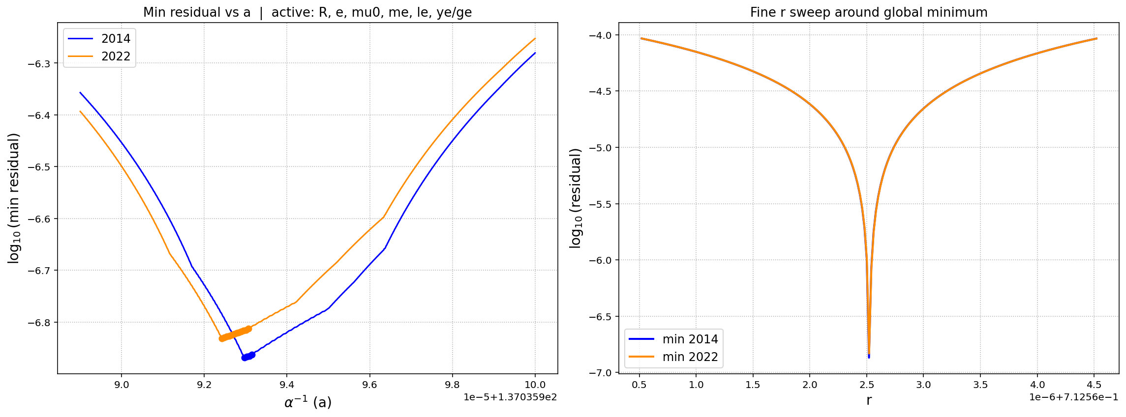
\[ v =\frac{c}{2 \pi \Omega^2} \]Using the CODATA values for the 6 most precise constants \(e^*, (y_e/g_e)^*, \lambda_e, m_e^*, R^*, \mu_0^*\) to tune our results, we can determine the optimal aggregate values for \(a\) and \(r\), \(h\) has no \(\alpha\) and so is not included lest it skew the output. We ran a simulation program, it weighs each constant equally within \(a\) and \(r\) nested loops, and then averages the results (fig 1.).
CODATA 2014 values
\(e, R, \mu_0, m_e, y_e, \lambda_e\)
Global best: a = 137.03599297 r = 0.71256252 (CODATA 2014 values)
Global best: a = 137.03599243 r = 0.712562521 (CODATA 2022 values)
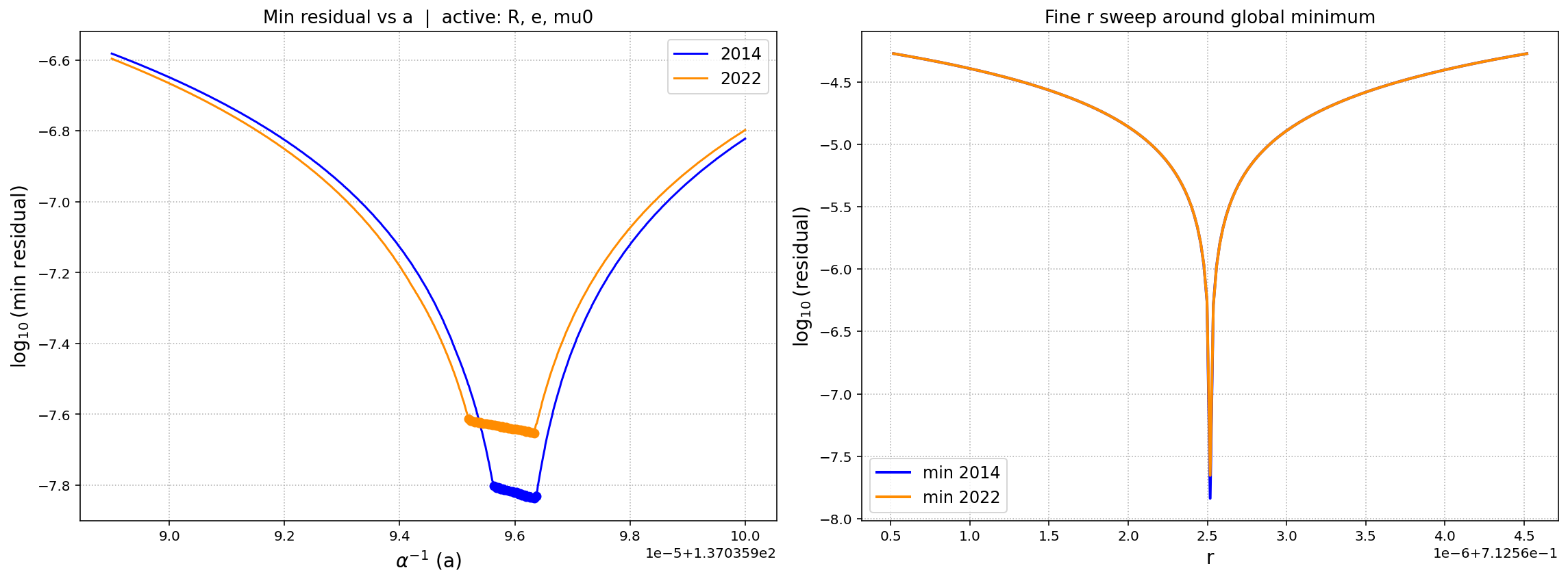
We can note that our constants can be divided into 2 groups;
Fig 2. \(e, R, \mu_0\)
Global best: a = 137.03599634, r = 0.7125625174 (CODATA 2014 values)
Global best: a = 137.03599634, r = 0.7125625174 (CODATA 2022 values)
Fig 3. \(m_e, y_e, \lambda_e\)
Global best: a = 137.03599296, r = 0.712562520 (CODATA 2014 values)
Global best: a = 137.03599242, r = 0.712562521 (CODATA 2022 values)
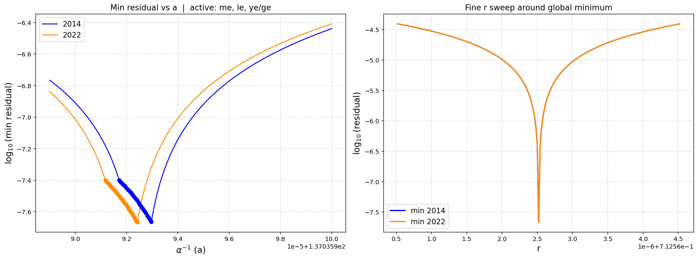
This is an indication that we cannot assign to each constant equal weights as the results (fig 1.) are skewed in favour of the \(m_e, y_e, \lambda_e\) group.
In the above we used \(c\) as an anchor and floating variables \(a\) and \(r\) in nested loops to correlate with the CODATA data. The model assigns to each unit an integer unit number (\(\theta; \theta=15 (kg), \theta=-13 (m), \theta=-30 (s)\) ... ). To validate this association, here we define the constants using combinations that incorporate the highest precision CODATA 2014 constants \(c\), \(\mu_0\), \(r\). This demonstrates the flexibility of the model and also serves to cross-check that unit number relationship. We first look for combinations in which the unit numbers are equal, and then add dimensionless components as required, table 3. For example; \(h^3\), \(\theta = 19*3 = 57\)
\[ {(h^*)}^3 = (2^3 \pi^4 \Omega^4 \frac{r^{13} u^{19}}{v^5})^3 = \frac{2^9 \pi^{12} \Omega^{12} r^{39}u^{57}}{v^{15}},\; \theta = 57 \] \[ \frac{2\pi^{10} {(\mu_0^*)}^3} {3^6 {(c^*)}^5 a^{13} {(R^*)}^2} = \frac{3^{19} \pi^{12} \Omega^{12} r^{39} u^{57}}{v^{15}},\; \theta = 57 \]We then replace the geometrical object with the numerical SI (\(c\), \(\mu_0\), \(r\), table 4.)
\[ {(h^*)}^3 = \frac{2\pi^{10} {\mu_0}^3} {3^6 {c}^5 a^{13} {R}^2} \]| Formula* | \(\theta\) (\(c\), \(\mu_0\), \(R\) formula units) | alpha |
|---|---|---|
| \((h^*)^3 = \displaystyle\frac{2\pi^{10} \mu_0^3}{3^6 c^5 a^{13} R^2}\) | \(\dfrac{\text{kg}^3}{\text{A}^6\,\text{s}}\), \(15\!\times\!3-3\!\times\!6+30 = 57\) | \(a\) =137.0359948156 |
| \((G^*)^5 = \displaystyle\frac{\pi^3 \mu_0}{2^{20} 3^6 a^{11} R^2}\) | \(\dfrac{\text{kg}\,\text{m}^3}{\text{A}^2\,\text{s}^2}\), \(15-13\!\times\!3-3\!\times\!2+30\!\times\!2 = 30\) | \(a\) =137.0212258623 |
| \((e^*)^3 = \displaystyle\frac{4\pi^5}{3^3 c^4 a^8 R}\) | \(\dfrac{\text{s}^4}{\text{m}^3}\), \(-30\!\times\!4+13\!\times\!3 = -81\) | \(a\) =137.0359956267 |
| \((k_B^*)^3 = \displaystyle\frac{\pi^5 \mu_0^3}{3^3 2 c^4 a^5 R}\) | \(\dfrac{\text{kg}^3}{\text{s}^2\,\text{A}^6}\), \(15\!\times\!3+30\!\times\!2-3\!\times\!6 = 87\) | \(a\) =136.9681945921 |
| \((m_e^*)^3 = \displaystyle\frac{16\pi^{10} R \mu_0^3}{3^6 c^8 a^7}\) | \(\dfrac{\text{kg}^3\,\text{s}^2}{\text{m}^6\,\text{A}^6}\), \(15\!\times\!3-30\!\times\!2+13\!\times\!6-3\!\times\!6 = 45\) | \(a\) =137.0359910965 |
| \((l_p^*)^{15} = \displaystyle\frac{\pi^{22} \mu_0^9}{2^{35} 3^{24} a^{49} c^{35} R^8}\) | \(\dfrac{\text{kg}^9\,\text{s}^{17}}{\text{m}^{18}\,\text{A}^{18}}\), \(15\!\times\!9-30\!\times\!17+13\!\times\!18-3\!\times\!18 = -195\) | \(a\) =137.0310051475 |
| \((m_P^*)^{15} = \displaystyle\frac{2^{25} \pi^{13} \mu_0^6}{3^6 c^5 a^{16} R^2}\) | \(\dfrac{\text{kg}^6\,\text{m}^3}{\text{s}^7\,\text{A}^{12}}\), \(15\!\times\!6-13\!\times\!3+30\!\times\!7-3\!\times\!12 = 225\) | \(a\) =137.0512385150 |
By reorganizing the constants into unit-free, scalar-free combinations, both the model unit numbers and the two SI translation scalars cancel. These combinations are not generally dimensionless in ordinary SI units; rather, they are dimensionless in the unit-number geometry, with \(\theta=0\). This distinction is important because in combinations where both units and scalars cancel, the SI constants should return the same numerical values as the \(MTP\alpha\) analogues. If the \(MTP\alpha\) objects are natural units, then in dimensionless combinations the SI constants will shed their scalar components, and reduce to the underlying embedded \(MTP\) objects (e.g.: \(c = V v = 299792458\) m/s and thus sans scalar \(v\), \(c = V = 2\pi \Omega^2\)).
Here we consider seven combinations of CODATA constants (dimensionless according to the unit‑number model; \(\theta = 0\), dimensioned according to the SI system). Except for no.7, each combination comprises the 2 fixed constants \(c, \mu_0\) and 1 high‑precision constant. As with the previous section, we first convert the constants into their geometric analogues and then move the alpha component to the right hand side of the equation (table 4). The table uses CODATA 2014, however combination no.7 is compared with CODATA 2022.
\[ \begin{aligned} R_1 &= \frac{e^7 c^{21}}{\mu_0^3} &&\text{SI: } \mathrm{kg^{-3}\,m^{18}\,s^{-8}\,A^{13}},\; \theta = (-27)\cdot7 + 17\cdot21 - 56\cdot3 = 0\\[6pt] R_2 &= \frac{\lambda_e^7 c^{35}}{\mu_0^9} &&\text{SI: } \mathrm{kg^{-9}\,m^{33}\,s^{-17}\,A^{18}},\; \theta = (-13)\cdot7 + 17\cdot35 - 56\cdot9 = 0\\[6pt] R_3 &= \frac{R_\infty^7 \mu_0^9}{c^{35}} &&\text{SI: } \mathrm{kg^{9}\,m^{-33}\,s^{17}\,A^{-18}},\; \theta = 13\cdot7 + 56\cdot9 - 17\cdot35 = 0\\[6pt] R_4 &= \frac{h^7 c^{35}}{\mu_0^{13}} &&\text{SI: } \mathrm{kg^{-6}\,m^{36}\,s^{-16}\,A^{26}},\; \theta = 19\cdot7 + 17\cdot35 - 56\cdot13 = 0\\[6pt] R_5 &= \left(\frac{y_e}{g_e}\right)^7 \mu_0 c^{14} &&\text{SI: } \mathrm{kg^{-6}\,m^{15}\,s^{-9}\,A^{5}},\; \theta = (-42)\cdot7 + 56\cdot1 + 17\cdot14 = 0\\[6pt] R_6 &= \frac{m_e^7 c^{7}}{\mu_0^4} &&\text{SI: } \mathrm{kg^{3}\,m^{3}\,s^{1}\,A^{8}},\; \theta = 15\cdot7 + 17\cdot7 - 56\cdot4 = 0\\[6pt] R_7 &= R^{21} \mu_0^{12} e^{35} &&\text{SI: } \mathrm{kg^{12}\,m^{-9}\,s^{11}\,A^{11}},\; \theta = 13\cdot21 + 56\cdot12 - 27\cdot35 = 0 \end{aligned} \]| Expression | Value |
|---|---|
| \(e\) | \(\left( \dfrac{2^{103} \pi^{64} \Omega^{75}}{R_1} \right)^{1/10}\) = 137.0359949837 |
| \(\lambda_e\) | \(\left( \dfrac{R_2}{2^{288} \pi^{157} 3^{21} \Omega^{225}} \right)^{1/12}\) = 137.0359924297 |
| \(R\) | \(\left( \dfrac{1}{2^{295} \pi^{157} 3^{21} \Omega^{225} R_3} \right)^{1/26}\) = 137.0359963688 |
| \(h\) | \(\left( \dfrac{2^{199} \pi^{128} \Omega^{150}}{R_4} \right)^{1/13}\) = 137.0359927447 |
| \(\gamma_e\) | \(\left( \dfrac{R_5}{2^{178} \pi^{86} 3^{21} \Omega^{150}} \right)^{1/15}\) = 137.0359915771 |
| \(m_e\) | \(\left( \dfrac{1}{2^{89} \pi^{29} 3^{21} \Omega^{75} R_6} \right)^{1/25}\) = 137.0359929242 |
| \(G\) | \(\left( \dfrac{1}{2^{89} \pi^{29} 3^{21} \Omega^{75} R_6} \right)^{1/25}\) = 137.0359929242 |
| \(k_B\) | \(\left( \dfrac{1}{2^{89} \pi^{29} 3^{21} \Omega^{75} R_6} \right)^{1/25}\) = 137.0359929242 |
| \(Re2014\) | \(\left( \dfrac{1}{2^{370} \pi^{151} 3^{63} \Omega^{300} R_7} \right)^{1/128}\) = 137.0359958277 |
| \(Re2022\) | \(\left( \dfrac{1}{2^{370} \pi^{151} 3^{63} \Omega^{300} R_7} \right)^{1/128}\) = 137.0359955214 |
If the geometric model correctly describes nature then there are no dimensioned components (\(v\) and \(r\) have cancelled) to include in the calculations and so each (CODATA / Geometrical object) should closely approach unity at the model's residual scale (sans scalars the CODATA combination is the Geometrical object combination). This serves to validate the conjecture that the geometrical objects \(M=1, T=\pi, P=\Omega\) are natural Planck units, the above combinations would reduce to the same numerical values regardless of the system of units used;
“...ihre Bedeutung für alle Zeiten und für alle, auch außerirdische und außermenschliche Kulturen notwendig behalten und welche daher als »natürliche Maßeinheiten« bezeichnet werden können...”
...These necessarily retain their meaning for all times and for all civilizations, even extraterrestrial and non-human ones, and can therefore be designated as "natural units"... -Max Planck [10]
The Boltzmann constant \(k_B\) appears in two distinct measurement contexts in this analysis.
We may propose \(k_B^{**}\), derived as an electromagnetic constant by using the electron gyromagnetic ratio \(y_e = \gamma_e/2\pi = 28\,024\,951\,640(170)\) units = \(\text{kg}^{-1}\,\text{s}\,\text{A}\) (\(-15 + (-30) + 3 = -42\)) and the \(g\)-factor \(g_e = -2.00231930436182(52)\). This \(k_B^{**}\) closely matches the geometrical \(k_B^*\) :
\[ k_B^{**} = \frac{g_e h}{4\pi c y_e m_e} = 1.379\,510\,310(24) \times 10^{-23},\;\theta = 19 - 17 - (-42) - 15 = 29 \]Rewriting the above formula gives
\[ k_B^{**} = \left(g_e \cdot 2^3\pi^4 \Omega^4 r^{13}/v^5\right) \big/ \left(4\pi \cdot 2\pi\Omega^2 v \cdot y_e \cdot (1r^4/v)/\psi\right) \]The thermal \(k_B\) discrepancy may indicate that the present electromagnetic‑geometric mapping is not capturing the thermodynamic temperature sector, or that \(k_B^*\) corresponds to a different electromagnetic scale rather than the macroscopic thermodynamic Boltzmann constant.
Note: \(k_B^{**}\) is not the thermodynamic Boltzmann constant measured by macroscopic thermometry. It is a model‑defined electromagnetic scalar constructed from electron‑sector quantities and not an independent CODATA measurement of the thermal Boltzmann constant.
The results in Section 4 reveal that within this geometric framework, the dimensioned constants are not mathematically independent, but are tightly coupled projections of a single underlying structure parametrized by \(\alpha\). This perspective offers insights into the fundamental nature of the constants, their relative precisions, and how they should be evaluated experimentally.
The dimensionless combinations in Section 4.3 (and the explicit parametrizations in Section 4.2) demonstrate that \(\alpha\) can be extracted from ostensibly unrelated constants. Because \(\alpha\) acts as the primary geometric scaling factor, the physical constants collectively “vote” on its value. The equations act as a magnifying glass for precision, revealing a profound physical pattern: a clear delineation between “bare” fundamental constants and “dressed” statistical constants.
The constants that fit perfectly with the consensus \(\alpha\) (e.g., \(e, h, m_e, \lambda_e\)) share a common trait: they are intrinsic quantum properties of single particles or the pure vacuum. They yield \(\alpha\) values tightly clustered. Conversely, the constants that cause the greatest deviation (yielding values like \(137.02\) and \(136.96\)) are the Boltzmann constant (\(k_B\)) and the gravitational constant (\(G\)).
The deviating constants do not, however, form a single group, and the distinction matters. Propagating each constant's own CODATA uncertainty through the relevant root gives the deviation in units of that uncertainty:
| constant | relative uncertainty | propagated \(\delta\alpha^{-1}\) | deviation |
|---|---|---|---|
| \(G\) | \(4.6\times10^{-5}\) | \(2.9\times10^{-3}\) | \(5.1\sigma\) |
| \(\ell_P\) | \(2.4\times10^{-5}\) | \(9.9\times10^{-4}\) | \(5.1\sigma\) |
| \(m_P\) | \(2.3\times10^{-5}\) | \(3.0\times10^{-3}\) | \(5.1\sigma\) |
| \(k_B\) | \(5.7\times10^{-7}\) | \(4.7\times10^{-5}\) | \(1441\sigma\) |
\(G\), \(\ell_P\) and \(m_P\) deviate by the same \(5.1\sigma\), and they are not independent: \(\ell_P\) and \(m_P\) are defined through \(G\), so a single poorly-determined input carries all three. A common offset of this size and consistency is what one expects if the recommended \(G\) is low by roughly one part in \(10^{4}\), and it is better read as a prediction about \(G\) than as three separate failures.
\(k_B\) is a different case. Its relative uncertainty is two orders smaller than \(G\)'s, so its deviation amounts to some \(1441\sigma\) and cannot be attributed to measurement imprecision. The statistical-averaging argument advanced above is aimed at the right constant, but the magnitude of the discrepancy shows how much that argument must carry; the electromagnetic construction of \(k_B^{**}\) in Section 4.4 is the more substantive response, and the reader is referred there.
The two cases should not be merged. “Macroscopically measured constants deviate” is correct for the \(G\) family and, at \(1441\sigma\), insufficient for \(k_B\).
Further supporting this is the derivation of \(k_B^{**}\) in Section 4.4, which is constructed entirely from the electromagnetic and electron-sector parameters (e.g., \(g_e, y_e, h, m_e\)). This structural link suggests that the scaling of temperature and entropy at the quantum level is not an independent thermodynamic primitive, but possesses a fundamental electromagnetic origin tied to the same geometric lattice. In Article 1a on measuring the CMB, temperature is a function within the radiation domain.
CODATA determines the recommended values of the constants using a Least Squares Adjustment (LSA), which treats the constants as independent variables constrained only by established physical laws (e.g., \(R_\infty = \alpha^2 m_e c / 2h\)).
However, if the universe operates on an overdetermined geometric lattice, this assumption of fundamental independence is flawed. By adjusting constants as if they are free parameters, the LSA effectively smears experimental errors across the parameter space. It forces consistency with macroscopic equations but artificially breaks the deeper geometric symmetries linking the constants.
The 2019 SI redefinition exacerbates this by meteorologically fixing \(h\), \(e\), and \(k_B\) to exact numerical values. By convention, this severs any underlying mathematical dependency between them. If the geometric model is correct, fixing these values based on 2018 experimental limits permanently misaligns the SI system from the true geometric lattice.
While the geometric model allows for various combinations of anchors to fully define the physical constants, practical metrology requires anchors that are highly precise and robustly realized in a laboratory. Historically, anchoring the electromagnetic sector to the vacuum permeability \(\mu_0\) relied on macroscopic, classical mechanical force measurements.
A far more precise and meteorologically practical approach is to replace \(\mu_0\) with the elementary charge \(e\). Anchoring the system to the trio of \(c\), \(R_\infty\), and \(e\) seamlessly bridges the kinematic, atomic, and quantum domains.
Crucially, the elementary charge is strongly preferred over the Planck constant (\(h\)) as the third anchor within this framework. Because the geometric analogue \(e^*\) natively contains an \(\alpha\) term (whereas \(h^*\) does not), utilizing \(e\) provides a direct mathematical cross-check on the fine-structure constant. By forming a combination of \(c\), \(R_\infty\), and \(e\) in which both the SI translation scalars (\(r, v\)) and the unit-number invariant (\(\theta = 0\)) perfectly cancel, the geometric lattice yields a direct algebraic relationship:
\[ R_\infty = \frac{c^5}{2^{28}3^3 \pi^{16} \Omega^{27}}\; \frac{1}{a^5 r^9} \] \[ e = \frac{2^{10} \pi^7 \Omega^9}{c^3} \; \frac{r^3}{a} \] \[ c^4 R_\infty e^3 = \frac{4\pi^5}{3^3 a^8} \]Rearranging this isolates the fine-structure constant into an elegant, low-exponent formula:
\[ \alpha^{-1} = \left( \frac{4\pi^5}{3^3 c^4 e^3 R_\infty} \right)^{1/8} \]If metrological institutions were to adopt \(c\), \(R_\infty\), and \(e\) as exact fixed values, this formulation would provide an analytically derived value for \(\alpha\). Once \(\alpha\) is defined, the remaining fundamental constants---such as \(h\), \(m_e\), and \(\mu_0\)---can be precisely calculated from the lattice without experimental uncertainty.
Validating this geometric framework does not require metrological institutions to immediately abandon their current adjustment methodologies. Instead, the model can be rigorously tested today by leveraging the constants that are already exact under the post-2019 SI system.
By adopting the exact 2022 values for \(c\) and \(e\), alongside the highly stable mean 2022 value for \(R_\infty\), the 8th-root formula yields a rigid, highly precise prediction for \(\alpha_{\text{model}}\). With this established, the geometric lattice outputs exact predictions for \(h\), \(m_e\), and \(\mu_0\). These derived values will exhibit slight deviations from the CODATA adjusted values, providing a falsifiable hypothesis (with the caveat that the measured values for \(c\), \(R_\infty\) and \(e\) are sufficiently independent of each other and of other constants).
A critical hurdle in testing these predictions is the reliance on theoretical corrections in standard metrology. The present CODATA \(\alpha\) is heavily weighted by calculations derived from Quantum Electrodynamics (QED) perturbation series, such as the 10th-order expansions used to extract \(\alpha\) from the electron anomalous magnetic moment (\(g_e\)).
If the geometric unit-number lattice represents a foundational structure of the physical constants, perturbative QED may merely be an asymptotic mathematical approximation of this deeper geometry.
To rigorously test the geometric model without circular bias, verification must rely strictly on raw, uncorrected experimental data from QED-independent physical phenomena. Promising avenues include:
Because the geometric model yields exact \(\theta = 0\) invariants for multiple combinations of constants, verification is not restricted to a single experimental regime. Instead, researchers can adopt an orthogonal testing strategy that actively isolates constants to avoid the “smearing” of experimental errors that occurs in global least-squares adjustments.
By strictly limiting the assumed variables, experiments can be categorized into two independent verification pathways:
This modular approach allows experimentalists to scour historical and contemporary literature for highly precise, narrow-scope experiments. More importantly, it establishes the ultimate consistency check: if the geometric unit-number lattice is the true physical foundation of the universe, then raw empirical data from Pathway A (blind to \(e\)) and Pathway B (blind to \(h\)) must independently converge on the exact same underlying \(\alpha\).
Using the CODATA 2022 values as a preliminary test, the convergence between these isolated pathways is exceptionally tight:
This allows the geometric framework to be validated from completely independent directions, entirely bypassing the need for interconnected CODATA adjustments.
The preceding sections establish numerical relationships. This section asks a different question: are they compressible, and by how much? The question is worth separating because it can be answered without reference to whether the geometric interpretation is correct. Given the constants as bare numbers, either a short rule reproduces them or it does not.
Any argument of this kind faces one objection above all others: that the expressions were found by trawling a large space of candidates, and that the description length omits the cost of the search. Minimum description length charges for a model's location in model-space, not only for its length. If the exponents in \(c^{4}R_\infty e^{3}\) were freely chosen, the search space would be enormous --- of order \(10^{6}\) expressions per target, some 20 bits each --- and no compression could survive it.
The exponents are not freely chosen. Scalar-freedom requires that both \(r\) and \(v\) cancel, and because \(\theta = 8a + 17b\), the unit-number cancels automatically once they do. This is two constraints, not three. A combination of three constants therefore satisfies a homogeneous \(2\times3\) system, whose integer solutions form a rank-one lattice: the exponents are the unique primitive null vector, determined up to sign and overall scaling.
Worked example. With scalar content \(r^{a}v^{b}\),
\[ c \to (0,1), \qquad R_\infty \to (-9,5), \qquad e \to (3,-3), \]the conditions \(\sum n_i a_i = 0\) and \(\sum n_i b_i = 0\) give
\[ -9n_2 + 3n_3 = 0, \qquad n_1 + 5n_2 - 3n_3 = 0 \quad\Longrightarrow\quad (n_1,n_2,n_3) = (4,1,3), \]that is, \(c^{4}R_\infty e^{3}\). This is the combination used in Section 6.3. Nothing was selected: given the three constants, the exponents follow, and the verification is a two-line calculation any reader can repeat.
Because the exponents are forced, the only freedom lies in choosing which constants to combine. The constants used in this paper are
\[ \{\,c,\ R_\infty,\ e,\ h,\ m_e,\ \lambda_e,\ \mu_0,\ y_e/g_e\,\}, \]with scalar content and unit numbers as follows:
| constant | \(a\) | \(b\) | \(\theta = 8a+17b\) |
|---|---|---|---|
| \(c\) | \(0\) | \(1\) | \(17\) |
| \(R_\infty\) | \(-9\) | \(5\) | \(13\) |
| \(e\) | \(3\) | \(-3\) | \(-27\) |
| \(h\) | \(13\) | \(-5\) | \(19\) |
| \(m_e\) | \(4\) | \(-1\) | \(15\) |
| \(\lambda_e\) | \(9\) | \(-5\) | \(-13\) |
| \(\mu_0\) | \(7\) | \(0\) | \(56\) |
| \(y_e/g_e\) | \(-1\) | \(-2\) | \(-42\) |
There are \(\binom{8}{3}=56\) triples, every one of which yields a non-trivial forced exponent vector. Five are degenerate: whenever both \(R_\infty\) and \(\lambda_e\) appear the third constant drops out with exponent zero, because \((-9,5)\) and \((9,-5)\) cancel as a pair. Six triples therefore collapse onto the single two-constant invariant
\[ R_\infty\lambda_e = \frac{\alpha^{2}}{2}, \]verified against CODATA 2022 to \(2\times10^{-12}\). This is the standard result obtained by combining \(R_\infty = \alpha^{2}m_ec/2h\) with \(\lambda_e = h/m_ec\); the lattice recovers it as the unique scalar-free pair, which is a check the model could have failed rather than a new relation.
Discounting the degeneracy leaves \(51\) distinct combinations, so the search freedom is
\[ \log_2 51 = 5.7\ \text{bits}, \]against the \(\sim124\) bits that free exponents would have cost. The table below lists a representative selection, including the three pathways used in Sections 4 and 7; the remainder follow by the same two-line construction.
| constants | exponents | combination |
|---|---|---|
| \(c,R_\infty,e\) | \((4,1,3)\) | \(c^{4}R_\infty e^{3}\) |
| \(c,R_\infty,h\) | \((20,-13,-9)\) | \(c^{20}R_\infty^{-13}h^{-9}\) |
| \(c,R_\infty,m_e\) | \((11,-4,-9)\) | \(c^{11}R_\infty^{-4}m_e^{-9}\) |
| \(c,e,h\) | \((24,13,-3)\) | \(c^{24}e^{13}h^{-3}\) |
| \(c,e,m_e\) | \((9,4,-3)\) | \(c^{9}e^{4}m_e^{-3}\) |
| \(c,e,\lambda_e\) | \((4,3,-1)\) | \(c^{4}e^{3}\lambda_e^{-1}\) |
| \(c,h,m_e\) | \((7,4,-13)\) | \(c^{7}h^{4}m_e^{-13}\) |
| \(c,h,\lambda_e\) | \((20,-9,13)\) | \(c^{20}h^{-9}\lambda_e^{13}\) |
| \(c,m_e,\lambda_e\) | \((11,-9,4)\) | \(c^{11}m_e^{-9}\lambda_e^{4}\) |
| \(R_\infty,e,h\) | \((6,5,3)\) | \(R_\infty^{6}e^{5}h^{3}\) |
| \(R_\infty,e,m_e\) | \((9,11,12)\) | \(R_\infty^{9}e^{11}m_e^{12}\) |
| \(R_\infty,h,m_e\) | \((7,11,-20)\) | \(R_\infty^{7}h^{11}m_e^{-20}\) |
| \(e,h,m_e\) | \((7,-9,24)\) | \(e^{7}h^{-9}m_e^{24}\) |
| \(e,h,\lambda_e\) | \((5,3,-6)\) | \(e^{5}h^{3}\lambda_e^{-6}\) |
| \(e,m_e,\lambda_e\) | \((11,12,-9)\) | \(e^{11}m_e^{12}\lambda_e^{-9}\) |
| \(h,m_e,\lambda_e\) | \((11,-20,-7)\) | \(h^{11}m_e^{-20}\lambda_e^{-7}\) |
| four further triples degenerate to \(R_\infty\lambda_e\) (see text) | ||
The trials factor is therefore \(5.7\) bits. This is not merely small; it is negligible beside every other term in the accounting, and the conclusion is unaffected by the exact size of the constant set --- adding two further constants moved the figure by \(1.6\) bits.
Specifying the six CODATA constants to their measured precision requires approximately 208 bits. The lattice specifies them from \(\Omega\), the \(\theta\)-algebra, the base-15 lock and two scalars. Costing the rule-set honestly is the least rigorous step, so we present the result as a function of it rather than as a single figure:
| rule-set (bits) | total (bits) | compression (bits) | factor |
|---|---|---|---|
| 80 | 126 | 82 | \(10^{25}\) |
| 100 | 146 | 62 | \(10^{19}\) |
| 120 | 166 | 42 | \(10^{13}\) |
| 140 | 186 | 22 | \(10^{6.5}\) |
| 160 | 206 | 2 | \(10^{0.5}\) |
| 180 | 226 | \(-18\) | \(10^{-5.5}\) |
Totals include 17 bits for the two scalars, 25 bits for the residuals, and 4.1 bits of search freedom from the enumeration above.
A costing of roughly 100 bits is defensible: the derived expressions chain rather than standing independently, since \(V\), \(L\), \(A\) and \(K\) follow from \(M\), \(T\), \(P\) by short rules. The compression is therefore real across the plausible range, but its magnitude is uncertain by many orders and should be quoted as a range.
Three structural choices (see Article 1b) carry information without carrying any adjustable number, and a strict accounting should name them even where it cannot cost them precisely.
None of these is a fitted parameter, and none can absorb a numerical discrepancy. But each locates the model within a space of alternatives, and an adversarial accounting would charge for that location. We estimate the three at perhaps 20--40 bits combined, which the table above already accommodates within its range.
It establishes compressibility. Six constants that are independently measured, and whose values carry no obvious relationship, are reproduced from a rule-set materially shorter than the data. This holds without reference to whether the geometric interpretation is correct: the compression is a property of the numbers.
It does not establish the mechanism. A short description is evidence that structure exists, not that this particular structure is the right one. Any equally short rule-set reproducing the same constants would have equal claim, and none is currently known.
The over-determination is the substantive part. Three of the six constants --- \(\lambda_e\), \(y_e/g_e\) and \(R_\infty\) --- are related to the others by standard physics.
\[ \lambda_e = \frac{h}{m_e c},\qquad \mu_0 = \frac{2 h}{e^2 c a},\qquad \frac{y_e}{g_e} = \frac{e}{4\pi m_e},\qquad R_\infty = \frac{\alpha^{2} m_e c}{2h}, \]The lattice reproduces those relations rather than assuming them, which is a constraint it could have failed; but the compression they contribute is not new information. What remains is the agreement among \(e\), \(h\) and \(m_e\), together with the derived \(\mu_0\), and it is that residual which carries the evidential weight.
The forced exponents are the strongest single point. If a critic grants nothing else, the null-space result of Section 6.1 still stands: the combinations were not selected from a large candidate set, because the candidate set has seventeen members and their exponents are determined by two linear constraints. That is checkable in a line, and it removes the objection that most often defeats numerological claims.
From compression to physical reality. It must be stated clearly that algorithmic compression establishes the existence of structure, not necessarily its physical mechanism. A sufficiently complex polynomial can fit any dataset. However, the model presented here does not fit a curve to data; it derives the data from a rigid, parameter-free geometric lattice constrained by a Diophantine null-space. The fact that a rule-set of roughly 100 bits can reproduce 208 bits of independent empirical data to a relative precision of \(10^{-9}\) strongly implies that the constants are not arbitrary empirical inputs, but are the compressed output of an underlying algorithmic geometry.
The analysis rests on three results that do not depend on one another. Each could hold while the others failed, which is why they are worth separating.
Convergence of orthogonal pathways. Two combinations of constants, chosen so that neither shares a measured input with the other, return values of \(\alpha^{-1}\) that agree far more closely with each other than either does with the recommended value:
| pathway | construction | \(\alpha^{-1}\) |
|---|---|---|
| A (kinematic, no \(e\)) | \(c^{40}/(R_\infty^{26}h^{18})\) | \(137.03599512277\) |
| B (electromagnetic, no \(h\)) | \(c^{4}R_\infty e^{3}\) | \(137.03599520395\) |
| difference | \(8.12\times10^{-8}\) | |
| relative | \(5.9\times10^{-10}\) | |
No parameter was fitted in either construction. The two pathways lie \(49\times\) closer to one another than either lies to the CODATA value, and their exponents are forced rather than chosen (Section 6.1). A third combination reinforces this. Taking the triple \(\{R_\infty, \mu_0, e\}\) --- which uses only one exact constant, and in which every term carries an explicit \(\alpha\) dependence --- the scalar-cancellation conditions of Section 6.1 return the exponents
\[ (n_{R}, n_{e}, n_{\mu_0}) = (21,\,35,\,12), \]giving \(R_\infty^{21}e^{35}\mu_0^{12}\) and \(\alpha^{-1} = 137.03599552\). These exponents were not selected: they are the unique primitive null vector of the \(2\times3\) system, exactly as for pathways A and B. The third pathway is therefore a further instance of the forced-exponent result rather than an independent numerical coincidence, and it agrees with the other two to \(4\times10^{-7}\) relative while all three remain some \(190\sigma\) from the recommended value.
These results are least vulnerable to the objection that \(\alpha\) was tuned, since nothing was tuned.
An out-of-sample determination of \(\mu_0\). In the two-parameter fit of Section 4, the permeability never enters the objective; it is forced once \(a\) and \(r\) are fixed. It reproduces \(4\pi\times10^{-7}\) to \(1.61\times10^{-9}\). Because every \(a_i\) is a monomial in \(\mathrm{\mu_0}\), each condition \(a_i=1\) fixes the same value, so the residual minimum is unique --- confirmed by scanning \(r\) over a range \(6\times10^{4}\) times the working window and finding one minimum. The location of the search window therefore cannot manufacture the result.
Compressibility. The six constants are reproduced from a rule-set materially shorter than the data, with the candidate set containing seventeen members rather than the \(10^{6}\) that free exponents would allow. The compression factor is uncertain by many orders --- between \(10^{0.5}\) and \(10^{25}\) across plausible rule-set costings --- but it is positive across that range, and it does not depend on the geometric interpretation being correct.
These results agree on a value of \(\alpha^{-1}\) near \(137.0359952\). The CODATA 2022 recommendation is \(137.035999177(21)\). The difference is \(4.01\times10^{-6}\), or \(191\sigma\) on the recommended uncertainty and this difference has significant implications but is not necessarily indicative of failure. The geometric \(\alpha\) represents a 'bare' lattice value, whereas the CODATA \(\alpha\) is a 'dressed' value altered by virtual loops.
The most precise readings of the 'geometric' alpha are derived solely via dimensionless combinations of the highest precision dimensioned constants. The recommended \(\alpha\) is dominated by determinations that use perturbative QED as an intermediary, whereas the geometric \(\alpha\) is QED-independent by construction. QED-free experimental data (following section) could further illuminate on reasons for this divergence. A key caveat is that the chosen constants must be independent of each other, yet clearly they share units, and so fixing the value of \(c\) may influence the readings of the other constants, for example it defines the meter. Hence multiple combinations need to be referenced and compared.
A QED-free determination of \(\alpha\). The quantum Hall effect yields \(\alpha\) directly through \(\alpha = \mu_0 c/2R_K\), with no perturbative input. Present determinations of this kind carry uncertainties near \(3\times10^{-6}\), which is comparable to the entire discrepancy: they are consistent with both values and cannot discriminate. To separate them at three standard deviations would require an uncertainty below \(1.34\times10^{-6}\), that is \(9.8\times10^{-9}\) relative --- roughly a factor of \(2.4\) beyond the best current value. That is a definite experimental target, not an aspiration.
Atom-recoil determinations already constrain the model. Measurements based on \(h/m\) reach \(10^{-11}\) relative and agree with the recommended value. They are QED-light rather than QED-free, but the margin is large: on reading (3) above, this agreement must be explained, and we cannot currently explain it. This is the sharpest existing tension.
Failure of the forced relations. The lattice reproduces \(\lambda_e = h/m_ec\), \(y_e/g_e = e/4\pi m_e\) and \(R_\infty\lambda_e = \alpha^{2}/2\) as consequences rather than inputs. Had any of these come out wrong the model would already be refuted, and they remain a live constraint as measurements improve.
The hierarchy identified in Section 5.1 — electromagnetic constants aligning tightly, macroscopic constants diverging — therefore functions as a built-in diagnostic: any future high-precision measurement that shifts a constant's derived \(\alpha\) toward or away from the geometric consensus will either validate or constrain the lattice. Constants with large or historically difficult measurements, such as \(G\) and the thermal Boltzmann constant, show larger discrepancies. Because the model is a rigid generative structure, once the scalars \(r\), \(v\), and the value of \(a\) are fixed, all remaining predictions are forced. For instance, if future acoustic gas thermometry or Johnson noise thermometry were to shift \(k_B\) toward the geometric \(k_B\), it would directly confirm the model's prediction that the current CODATA thermal \(k_B\) is biased by statistical averaging effects.
In this sense the model can be used as an anomaly detector for metrology and for the model itself. A constant whose measured value lies far from the model's prediction is flagged either as a possible metrological/systematic outlier or as a point where the present geometric model must be revised.
Of particular note, the most physically consequential part of the model is not merely that several constants can be numerically compressed, but that the electron sector appears to be generated by a single dimensionless invariant, \(\psi\) [1]. In this framework, the electron is not introduced as an independent particle with separately fitted mass, charge, wavelength, Rydberg linkage, and gyromagnetic scale. Instead, these quantities emerge as different dimensional projections of the same underlying geometric construction.
The invariant
\[ \psi=\frac{\sigma_e^3}{2T} =4\pi^2\left(2^6\cdot3\cdot\pi^2\cdot a\cdot\Omega^5\right)^3, \qquad a=\alpha^{-1}, \]is dimensionless: both the unit-number bookkeeping and the SI translation scalars cancel exactly. This is a stronger statement than an ordinary numerical fit. It means that the model assigns the electron a purely mathematical core, while the observed dimensional quantities arise only after the geometric object is translated into SI through the two scalars \(r\) and \(v\).
This provides a natural explanation for why several high-precision electron constants move together. The electron mass \(m_e\), Compton wavelength \(\lambda_e\), Rydberg constant \(R_\infty\), and gyromagnetic combination \(y_e/g_e\) are not independent in the model; they are linked by the same \(\psi\)-based construction. Therefore, repeated agreement among these constants should not be counted as fully independent statistical evidence. Instead, their shared residual pattern is itself a diagnostic: it tests whether one electron invariant can simultaneously organize the electron-sector constants.
If the \(\psi\) construction is physically meaningful, then the electron is not a primitive empirical input but a derived geometric object. Charge, mass, wavelength, and magnetic response become different appearances of the same dimensionless mathematical entity after projection into the SI unit system. This would shift the role of the electron from a measured building block to a structural bridge between the dimensionless \(MTP\) geometry and the observed constants of electromagnetism.
The proposed magnetic-monopole decomposition of \(\psi\), in which the electron is represented by three \(AL\)-type constituents forming a \(DDD\) structure, should be treated at present as a model-internal geometric interpretation rather than an established particle-physics result. Nevertheless, it gives the framework a concrete internal mechanism: the electron is not merely fitted by the constants, but constructed from the same base-15 unit-number rules that determine the rest of the lattice.
In this sense, the electron is the central falsifiable object of the model. The Planck-object construction supplies the geometric stage, the base-15 rule supplies the lattice constraint, and \(\Omega\) supplies the mathematical scale; but \(\psi\) is where the framework first becomes a particle model. If future precision measurements preserve the common electron-sector residual structure, the case for a genuine geometric electron strengthens. If they break the \(\psi\)-linked pattern, the model will require revision at its most fundamental physical point.
[1] Macleod, Malcolm J. "The Programmer God, are we in a simulation?" theprogrammergod.com
[2] Macleod, M.J. Programming Planck units from a virtual electron: a simulation hypothesis. Eur. Phys. J. Plus 133, 278 (2018). https://doi.org/10.1140/epjp/i2018-12094-x
[3] Macleod, Malcolm J., 1. Planck unit scaffolding to Cosmic Microwave Background correlation https://www.doi.org/10.2139/ssrn.3333513
[4] Macleod, Malcolm J., 2. Relativity as the mathematics of perspective in a hyper-sphere universe https://www.doi.org/10.2139/ssrn.3334282
[5] Macleod, Malcolm J., 3. Gravitational orbits from n-body rotating particle-particle orbital pairs https://www.doi.org/10.2139/ssrn.3444571
[6] Macleod, Malcolm J., 4. Geometrical origins of quantization in H atom electron transitions https://www.doi.org/10.2139/ssrn.3703266
[7] Macleod, Malcolm J., 5. Atomic Transitions via a Photon-Orbital Hybrid https://www.doi.org/10.13140/RG.2.2.10680.20487
[8] Macleod, Malcolm J., 6. Natural Planck units MTP and the Fine Structure Constant Alpha https://www.doi.org/10.2139/ssrn.4346640
[9] Macleod, Malcolm J., 7. Geometric Origin of Quarks, the Mathematical Electron extended https://www.doi.org/10.13140/RG.2.2.21695.16808
[10] Macleod, Malcolm J., 8. Holographic Emergence in the Simulation Hypothesis https://www.doi.org/10.13140/RG.2.2.20919.28320
[14] Macleod, Malcolm J., 1b. Supplement: The Minimal Complexity Algorithm of the Planck Scaffolding https://www.doi.org/10.13140/RG.2.2.12830.09283/1
[15] Macleod, Malcolm J., 1c. Supplement: Heavens and the free-will postulate https://www.doi.org/10.13140/RG.2.2.32962.75200/1
[11] U. D. Jentschura and I. Nándori, “Attempts at a determination of the fine-structure constant from first principles: a brief historical overview” (2014). https://arxiv.org/abs/1411.4673
[12] Yoshio Koide, “What Physics Does The Charged Lepton Mass Relation Tell Us?” (2018); Zhi‑zhong Xing and He Zhang, “On the Koide‑like Relations for the Running Masses of Charged Leptons, Neutrinos and Quarks” (2006). https://arxiv.org/abs/1809.00425, https://arxiv.org/abs/hep-ph/0602134
[13] Particle Data Group, “Grand Unified Theories” (2024 review). https://pdg.lbl.gov/2024/reviews/rpp2024-rev-guts.pdf