We present a geometric model of hydrogen electron transitions built from the fine structure constant \(\alpha\), \(\pi\), and the reduced Compton wavelength of the electron--proton reduced mass. Orbitals are treated as rotating structures that evolve in discrete steps, one per \(\tau\)-loop of the atom. Transition involves a photon-orbital hybrid mediated by the electron in a 2-photon process (deletion of the current orbital with simultaneous absorption of the new orbital). The transition phase \(\Phi(n) = 4\pi(1-1/n)\) integrates an \(r^{-3/2}\) rotation law with a constant radial increment; divided by \(\pi\) it is a pure rational number, reaching exactly \(4\pi\) at ionization. With reduced Compton wavelengths the model reproduces the Bohr angular momentum \(L = n\hbar\) exactly, the reduced mass cancelling identically. Transition frequencies reproduce the reduced-mass Rydberg formula exactly; their residual against experiment is the relativistic fine structure and the Lamb shift, which the model does not contain. The fine structure depends on \(\alpha\) alone, and deriving it from the geometry is identified as the model's next project. The main argument does not invoke wavefunctions or the Schrödinger equation.
The quantization of atomic energy levels, first proposed by Bohr in 1913, remains one of the foundational mysteries of quantum mechanics. While the Schrödinger equation successfully predicts atomic spectra, it treats quantization as a mathematical requirement rather than explaining why energy levels must be discrete. The Schrödinger equation tells us what happens, but not why it happens. The question "Why are energy levels discrete?" is answered by postulating that wavefunctions must satisfy certain mathematical constraints, but the physical mechanism underlying this discreteness remains unclear.
The fine structure constant, \(\alpha \approx 1/137.036\), appears throughout atomic physics as the coupling strength between electromagnetic radiation and matter. Traditionally viewed as a dimensionless combination of fundamental constants (\(\alpha = e^2/4\pi\epsilon_0\hbar c\)), its geometric significance has remained obscure. Similarly, Compton wavelengths (\(\lambda_e\) for electrons, \(\lambda_p\) for protons) are typically interpreted as quantum mechanical length scales where particle-wave duality becomes important, yet their role in atomic structure is not fully explored in conventional treatments.
We propose that atomic quantization can be understood as a purely geometric phenomenon. Our model is based on the following minimal assumptions:
The model produces testable predictions about transition timescales and intermediate states that differ from standard quantum mechanics while reproducing its successful predictions for energy levels.
This approach applies Occam's razor: rather than postulating wavefunctions, operators, and quantization rules, we derive atomic behaviour from geometric constraints. Electrons end up in certain energy levels because geometry doesn't allow any other stable configurations. It's like how you can only fit certain numbers of people around a circular table—the constraint comes from the geometry, not from a rule.
Discrete particles in this model are replaced by a continuous electric wave-state to mass point-state oscillation.
Electric wave-state: Duration = particle frequency (measured in Planck time units). Position undefined; particle exists as extended wave.
Mass point-state: Duration = one Planck time \(t_p\). Position can be defined as a point.
The final particle frequency:
\[ f_{\text{particle}} = (\text{wave-state frequency} + 1) t_p \]The electron's wave-to-point cycle lasts \(\psi_e = m_P/m_e \approx 2.39\times10^{22}\) Planck times -- its reduced Compton period \(\bar\lambda_e/c\). With approximately \(1.85\times10^{43}\) Planck times in one second, this gives \(\approx 7.8\times10^{20}\) cycles per second. (The full Compton period \(\lambda_e/c = 2\pi\psi_e \approx 1.5\times10^{23}\,t_P\) is larger by \(2\pi\); this accounts for the figures \(10^{23}\) and \(2.4\times10^{22}\) quoted in different articles of this series, which refer to different quantities rather than conflicting.) This is a constant repeating oscillation and not a duality: the particle exists over time, and baryonic matter does not exist as a defined entity at unit Planck time (events occur at unit time in the Planck scale but are frequency dependent at the quantum scale). This artifice can be used to map both gravitational orbits and atomic orbital transitions as these 2 distinct particle states (wave and points) can replace forces (gravitational and electromagnetic).
Note (Domain Link): The mass point-state corresponds to the Matter (Integer) Domain where the particle has defined position and mass. The electric wave-state corresponds to the Radiation (\(\sqrt{\text{Integer}}\)) Domain where the particle exists as an extended wave (see Article 1 for domain definitions).
Throughout this article reduced Compton wavelengths \(\bar\lambda = \hbar/mc\) are used. The choice is not arbitrary: it is the one for which the model reproduces the Bohr angular momentum \(L = n\hbar\) exactly (Section 2.3), where the full wavelength would give \(L = nh\).
The fundamental length is the sum of the electron and proton reduced Compton wavelengths,
\[ \ell_0 = \bar\lambda_e + \bar\lambda_p = \frac{\hbar}{m_e c} + \frac{\hbar}{m_p c} = 3.8636957687\times10^{-13}\,\text{m}, \]with \(\bar\lambda_e = 3.8615926796\times10^{-13}\)\,m and \(\bar\lambda_p = 2.1030891034\times10^{-16}\)\,m.
This is not an ad hoc sum. Collecting terms,
\[ \ell_0 = \frac{\hbar}{c}\,\frac{m_e+m_p}{m_e m_p} = \frac{\hbar}{\mu c},\qquad \mu = \frac{m_e m_p}{m_e+m_p}, \]so \(\ell_0\) is exactly the reduced Compton wavelength of the reduced mass -- the single length belonging to the object that reduces the two-body problem to a one-body one. The reduced-mass correction of standard quantum mechanics is therefore not merely encoded in \(\ell_0\): \(\ell_0\) is the Compton length of the reduced mass, to \(1.3\times10^{-16}\).
One simulation step is the time light takes to cross this length, \(\tau_{\text{step}} = \ell_0/c = 1.288790\times10^{-21}\)\,s, which is exactly one \(\tau\)-loop of the hydrogen composite in the branch model of Article 1b.
The Bohr radius is \(a_0 = \alpha_{\text{inv}}\bar\lambda_e\) (inverse fine structure constant \(\alpha_{\text{inv}} \approx 137.03599\)...), and its reduced-mass counterpart is \(a_\mu = \alpha_{\text{inv}}\hbar/(\mu c) = 5.294654\times10^{-11}\)\,m. The model's orbital radius and velocity at shell \(n\), in units of \(\ell_0\) and of \(\ell_0\) per step, are
\[ r_n = 2\alpha_{\text{inv}}\,n^2,\qquad v_n = \frac{1}{2\alpha_{\text{inv}}\,n}, \]so the dimensionless ground-state radius is
\[ r_0 = 2\alpha_{\text{inv}}. \]Restoring units, \(r_n = 2\alpha_{\text{inv}}\ell_0 n^2 = 2a_\mu n^2\) and \(v_n = \alpha c/(2n)\): the model orbit has approximately twice the Bohr radius (Bohr radius uses \(\lambda_e\)) and half the Bohr velocity.
Angular momentum = \(n\hbar\). The product \(r_n v_n = n\) holds with \(\alpha_{\text{inv}}\) cancelling, so
\[ L = \mu\,r_n v_n = \mu\,(n\,\ell_0)\,c = \mu\,n\,\frac{\hbar}{\mu c}\,c = n\hbar . \]The reduced mass cancels exactly because \(\ell_0 = \hbar/\mu c\). The model therefore reproduces the Bohr quantization condition without assuming it.
Note. These formulas are applied in a simulation; however to reduce computation the length \(\ell_0\) is applied at the end, and so the following sections work primarily with the dimensionless components of the atom.
The radius of the orbital is \(r_{\text{orbital}}\). The angle of rotation is \(\beta_{\text{orbital}}\). This \(r_{\text{orbital}}^{-3/2}\) dependence is fundamental to the model as it determines the velocity of the orbital on a 2-D plane (representing 3-D space).
\[ \beta_{\text{orbital}} = \frac{1}{r_{\alpha} r_{\text{orbital}} \sqrt{r_{\text{orbital}}}} \] \[ r_{\alpha} = \sqrt{2 \alpha_{\text{inv}}} \]At the \(n = 1\) orbital, \(r_{\text{orbital}} = r_0\):
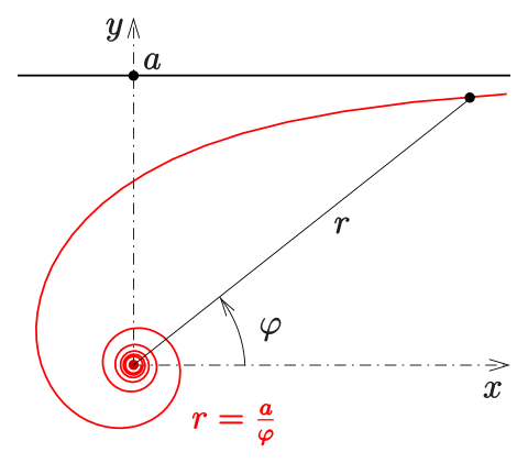
\[ \beta_{\text{orbital}} = \frac{1}{r_{\text{orbital}}^2} \]A hyperbolic spiral is a type of spiral with a pitch angle that increases with distance from its center. As this curve widens (radius \(r\) increases), it approaches an asymptotic line (the y-axis) with the limit set by a scaling factor \(a\) (as \(r\) approaches infinity, the y axis approaches \(a\)).
For the particular spiral that the electron transition path maps, periodically the spiral angles converge to give integer radius with \(4\pi\) as the limiting angle. Fig 1. is a general form for this type of spiral (beginning at the outer limit ranging inwards), this illustrates how the angle periodically returns an integer radius with \(4\pi\) as the limit;
\[ x = a^2 \frac{\cos(\varphi)}{\varphi^2},\; y = a^2 \frac{\sin(\varphi)}{\varphi^2},\;0 < \varphi < 4\pi \] \[ r = \sqrt{x^2 + y^2} \] \[ \varphi = (2)\pi, \; r = 4 \] \[ \varphi = (4/3)\pi,\; r = 9 \] \[ \varphi = (1)\pi, \; r = 16 \] \[ \varphi = (4/5)\pi, \; r = 25 \] \[ \varphi = (2/3)\pi, \; r = 36 \]As we note later, the electron spiral (which conversely begins inwards ranging outwards) follows the formula
\[ \varphi = 4\pi \left(1 - \frac{1}{n}\right) \]Strictly, the curve is a hyperbolic spiral in \(n = \sqrt{r/r_0}\) rather than in the radius itself. Writing \(\theta = 4\pi - \varphi\) for the angle remaining to the limit, the transition satisfies \(n\,\theta = 4\pi\) exactly -- the hyperbolic form \(n = 4\pi/\theta\) -- while the radius obeys \(r\,\theta^2 = 16\pi^2 r_0\), so that \(r \propto \theta^{-2}\). The equations above are of this second form; the figure shows the standard hyperbolic spiral \(r = a/\varphi\), which is the same curve with \(n\) taken as the radial coordinate.
We treat the orbital radius, not as a region of probability, but as a physical structure linking the proton and electron. It is this orbital radius which guides the rotation of the proton-electron orbital and the particles with it.
Picture the electron's orbit not as a continuous circle, but as a polygon with hundreds of thousands of sides—so many that it looks circular, but is actually made of discrete straight-line segments. Each segment corresponds to one wave-point oscillation cycle. The electron 'steps' around the orbit, taking about 472,000 steps to complete one revolution in the ground state (\(n=1\)).
Bohr model: When the electron is in an \(n\)-shell orbital (\(n\) is the principal quantum number), the model resembles the Bohr model albeit the rationale here being that the orbital rotates through discrete angular increments as defined by \(\beta\). In terms of the dimensionless component;
\[ r_{\text{orbital}} = r_0 n^2 = 2 \alpha_{\text{inv}} n^2 \] \[ \beta_{\text{orbital}} = \frac{1}{r_{\alpha} r_{\text{orbital}} \sqrt{r_{\text{orbital}}}} \]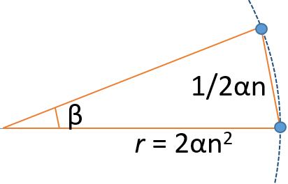
During the orbit, the electron is oscillating between the wave-state and the point-state. As only the point-state has defined co-ordinates, we are essentially mapping the orbital as a series of steps, the orbital arc length travelled by the electron per step equivalent to the inverse of the orbital radius.
\[ l_{\text{step}} = arc_{\text{step}} = \frac{1}{2 \alpha_{\text{inv}} n} \] \[ v_{\text{step}} = \frac{1}{2 \alpha_{\text{inv}} n} \]The number of steps for 1 complete rotation:
\[ t_{\text{orbital}} = 2\pi \frac{r_{\text{orbital}}}{v_{\text{orbital}}} = 2\pi r_{\text{orbital}} (2 \alpha_{\text{inv}} n) = 2\pi 2 \alpha_{\text{inv}} 2 \alpha_{\text{inv}} n^3 = 471964.36 (n^3) \]This number, derived purely from geometry, determines the entire model's timescale. Each step represents one oscillation at the Compton wavelength scale. We only require \(\alpha\) and \(\pi\), however we may also note that if the orbital is a polygon, then our \(\pi\) is also an approximation of \(\pi\) itself and so it may be possible to reduce further to \(\alpha\) and integers (these are provided by the universe expansion, Article 1).
The Lyman series energy formula can be decomposed:
\[ \frac{1}{\lambda} = R_\infty\left(1 - \frac{1}{n^2}\right) = R_\infty - \frac{R_\infty}{n^2} \]Mathematically (if not physically) we can divide into 2 waves:
\[ \text{Photon}_{n1} = R_\infty \] \[ \text{Photon}_{n\text{final}} = \left(- \frac{R_\infty}{n^2}\right) \] \[ \text{Photon}_{\text{total}} = \text{Photon}_{n1} + (-\text{Photon}_{n\text{final}}) \]This (mathematical) approach permits us to divide the transition into two distinct geometric processes taking place between the incoming photon and the orbital radius, with the electron taking the role as mediator. Rather than 2 actual distinct photons, we may presume two geometric phases of a single photon absorption, nevertheless the 2-photon image is easier to conceptualize. Note these processes are not instantaneous but rather occur over time in discrete steps;
Process 1 (Cancellation): A photon with energy corresponding to the \(n=1\) orbital frequency cancels the existing orbital structure.
\[ \text{Photon}_{n1} + \text{Orbital}_{n1} = \text{zero} \]Process 2 (Creation): A (-) photon with energy corresponding to the \(n_{\text{final}}\) orbital creates the new orbital structure.
\[ \text{Photon}_{n\text{final}} = \text{Orbital}_{n\text{final}} \]In terms of frequencies:
\[ \nu_{\text{transition}} = \nu_{n1} - \nu_{n\text{final}} = \nu_{n1}\left(1 - \frac{1}{n^2}\right) = \nu_{n1}\frac{n^2 - 1}{n^2} \]Orbital Phase (Duration: one orbit at \(n=1\)). The electron completes one orbit while the photon begins transferring momentum. During this phase, the \(n=1\) orbital is being 'cancelled' while the new orbital begins forming.
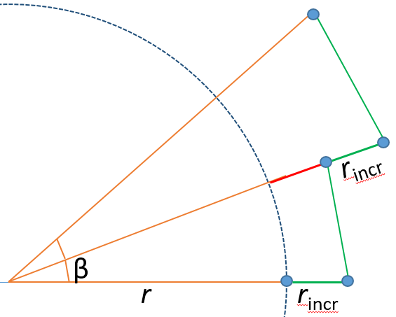
For the purpose of simulating the above we can represent each photon as a series of oscillation steps as we have done with the orbital. We can assign to each step a unit \(r_{\text{incr}}\) such that as \(\text{Photon}_{n1}\) merges with (is absorbed by) \(\text{Orbital}_{n1}\), the orbital radius (the radius of \(\text{Orbital}_{n1}\)) is reduced in \(r_{\text{incr}}\) steps.
\[ r_{\text{incr}} = \frac{-1}{2\pi 2 \alpha_{\text{inv}}} \]Conversely, because of the minus term, (-\(\text{Photon}_{n\text{final}}\)) adds to the orbital radius and so the electron completes 1 orbit with radius unchanged.
\[ r_{\text{orbital}} = r_{n1} + r_{\text{incr}} - r_{\text{incr}} \]However if we consider this process from the perspective of waveforms, we note that \(\text{Orbital}_{n1}\), the original orbital, has been cancelled (when it absorbed \(\text{Photon}_{n1}\)) leaving behind a partially absorbed (-\(\text{Photon}_{n\text{final}}\)). Here we define this as the orbital phase.
Absorption of a photon does not occur instantaneously but in gradual steps. For example, if (-\(\text{Photon}_{n\text{final}}\)) is equivalent to an \(n=2\) orbital (an \(\text{Orbital}_{n2}\)), then after the orbital phase, \((n^2 - 1)/n^2 = 3/4\) of (-\(\text{Photon}_{n\text{final}}\)) still remains to be absorbed. Here we define this absorption region as the transition phase.
Transition Phase (Duration: until \(n_{\text{final}}\) is reached). The orbital radius gradually expands through intermediate values between \(n=1\) and \(n=\text{final}\). The electron traces a spiral path during this phase. At the completion of the orbital phase the orbital radius begins to increase in steps of \(r_{\text{incr}}\):
\[ r_{\text{orbital}} = r_{\text{orbital}} - r_{\text{incr}} \]However the orbital itself also continues to rotate according to angle \(\beta\):
\[ \beta_{\text{orbital}} = \frac{1}{r_{\alpha} r_{\text{orbital}} \sqrt{r_{\text{orbital}}}} \]The total phase accumulated during the transition follows from the rotation law and the radial growth; it need not be found empirically. With \(\beta = 1/(r_\alpha r_{\text{orbital}}^{3/2})\), \(r_{\text{orbital}} = r_0 n^2\) and \(r_\alpha = \sqrt{r_0}\),
\[ \beta = \frac{1}{r_0^{2}\,n^{3}}, \]and the radius grows by one increment per step, so that \(n^2 = 1 + t/T_1\). Then \(dn/dt = 1/(2nT_1)\), and since \(T_1 = 2\pi r_0^2\),
\[ \frac{d\Phi}{dn} = \frac{\beta}{dn/dt} = \frac{2T_1}{r_0^2 n^2} = \frac{4\pi}{n^2}, \qquad \Phi(n) = \int_1^n \frac{4\pi}{n'^2}\,dn' = 4\pi\left(1 - \frac{1}{n_{\text{radius}}}\right). \]Numerical integration over the step sequence reproduces this to the precision of the arithmetic -- \(360.0000^\circ\), \(480.0000^\circ\) and \(540.0000^\circ\) for \(n = 2, 3, 4\). The hyperbolic spiral is therefore a consequence of the \(r^{-3/2}\) rotation law and the constant radial increment, not a curve fitted to the data. What remains postulated is the rotation law itself, carried over from the gravitational model of Article 3 with the constant \(\sqrt{2\alpha_{\text{inv}}}\).
Periodically the spiral angle returns an integer \(n_{\text{radius}}\). For example, the first 8 n-shells with transition angles \(\Phi\):
\[ \begin{align*} n = 1 \to 2: & \quad \Phi = 2\pi \quad \text{($r = 4 \times r_0$)} \\ n = 1 \to 3: & \quad \Phi = \frac{8\pi}{3} \quad \text{($r = 9 \times r_0$)} \\ n = 1 \to 4: & \quad \Phi = 3\pi \quad \text{($r = 16 \times r_0$)}\\ n = 1 \to 5: & \quad \Phi = \frac{16\pi}{5} \quad \text{($r = 25 \times r_0$)} \\ n = 1 \to 6: & \quad \Phi = \frac{10\pi}{3} \quad \text{($r = 36 \times r_0$)} \\ n = 1 \to 7: & \quad \Phi = \frac{24\pi}{7} \quad \text{($r = 49 \times r_0$)} \\ n = 1 \to 8: & \quad \Phi = \frac{7\pi}{2} \quad \text{($r = 64 \times r_0$)} \\ n = 1 \to \infty: & \quad \Phi \to 4\pi \quad \text{(ionization: $n_{\text{radius}} = \infty$)} \end{align*} \]By adding and rotating sections of \(\alpha\) in steps, a hyperbolic spiral emerges whose \(n\)-shell angles are functions of \(\pi\) alone and fall at the correct integer radius for each shell. The rotation law and the constant radial increment are the only inputs; the spiral, its dependence on \(\pi\), and the correspondence between angle and radius all follow from them.
The factor \(\pi\) enters from a single source: \(T_1 = 2\pi r_0^2\), the statement that one orbit is \(2\pi\). Divide it out and what remains is a pure rational number,
\[ \frac{\Phi(n)}{\pi} = 4\left(1 - \frac{1}{n}\right), \]so every transition phase is a rational multiple of \(\pi\) built from the integer \(n\) alone:
| \(n\) | 2 | 3 | 4 | 5 | 6 | 7 | 8 | \(\infty\) |
|---|---|---|---|---|---|---|---|---|
| \(\Phi/\pi\) | \(2\) | \(\tfrac83\) | \(3\) | \(\tfrac{16}{5}\) | \(\tfrac{10}{3}\) | \(\tfrac{24}{7}\) | \(\tfrac72\) | \(4\) |
Two features stand out. The \(1\to2\) transition sweeps exactly \(2\pi\), one complete turn. And the limit at ionization is exactly \(4\pi\), which is the rotation that returns a spin-\(\tfrac12\) state to itself (Section 3.6).
What the \(4\pi\) does and does not show. \(\Phi\) is an external rotation of the orbit, whereas spin concerns the electron's internal phase, and the two are related by the spin-\(\tfrac12\) half-angle. Read as a rotation, the complete ionizing transition is one spin-\(\tfrac12\) period and the \(1\to2\) transition (\(2\pi\)) is half of one. Read instead as internal phase, in half-cycles of \(\pi\), the \(1\to2\) transition is one period and ionization two. The readings differ by exactly the half-angle, and deciding between them requires knowing whether the orbital rotation drives the internal phase, which this article does not establish. The equality \(\Phi(\infty)=4\pi\) is exact; its connection to spin is recorded, not claimed.
The electron's wave-to-point cycle has the period of its reduced Compton wavelength, \(\bar\lambda_e/c = \psi_e t_P\), which is one \(\tau\)-loop in the branch model of Article 1b. Each loop advances the electron's internal phase by \(\pi\) rather than \(2\pi\):
\[ \omega_{\text{spin}}\,\frac{\bar\lambda_e}{c} = \pi , \]where \(\omega_{\text{spin}}\) is the rate of that internal phase. One loop therefore multiplies the state by \(e^{i\pi} = -1\), and a second restores it. For a spin-\(\tfrac12\) object a rotation through \(\theta\) contributes internal phase \(\theta/2\), so one loop corresponds to one full \(2\pi\) rotation and two loops to \(4\pi\): this is the double-valuedness of spin-\(\tfrac12\), arising from the half-cycle of the loop rather than being assumed.
Although \(n_{\text{radius}}\) is a measure of radius (in terms of the principal radius \(r_0\)), its usage is more commonly associated with the quantum number \(n\), and so by convention we will equate \(n = n_{\text{radius}}\), but in this model the principal quantum number \(n\) refers only to those set of integer states of \(n_{\text{radius}}\) periodically generated by the spiral.
The number of steps required for 1 complete orbital rotation at \(n = 1\):
\[ T_1 = 2\pi 2 \alpha_{\text{inv}} 2 \alpha_{\text{inv}} = 471964.36 \]The theoretical number of steps \(N_{\text{steps}}\) required to complete the transition (from start to end) becomes:
\[ N_{\text{steps}} = n^2 \times T_1 \]The transition frequency is defined as the inverse of one oscillation period at the Compton scale, multiplied by the geometric phase factor (including the dimensioned terms). During each oscillation cycle, the orbital radius changes by one geometric step (\(r_{\text{incr}}\)). The photon is fully absorbed when the radius reaches exactly \(n^2 \times r_0\), which happens after \(N_{\text{steps}} = n^2 \times T_1\) cycles. This gives:
\[ \nu_{1 \to n} = 2\,\frac{(n^2 - 1)}{N_{\text{steps}}}\,\frac{c}{\ell_0} = 2\left(1 - \frac{1}{n^2}\right)\frac{c}{T_1\ell_0}. \](In the full-wavelength form this reads \(4\pi(n^2-1)c/(N_{\text{steps}}\,\ell_{0,\text{full}})\); the two are numerically identical, since \(\ell_{0,\text{full}} = 2\pi\ell_0\).) The prefactor is the Rydberg frequency of the reduced mass,
\[ \frac{2c}{T_1\ell_0} = \frac{\alpha^2\mu c^2}{2h} = \frac{c\,R_\infty}{1+m_e/m_p}, \qquad \frac{2c}{\ell_0} = \frac{8\pi\alpha^{-2}R_\infty c}{1+m_e/m_p} = 1.551842981\times10^{21}\ \text{Hz}, \]so \(\nu_{1\to n}\) is the Bohr formula for the reduced mass, reached here by counting steps.
In the above we jumped between the orbital radius, spiral angle and quantum number \(n\), this is because in final analysis they are interchangeable. If we know 1 of these values then we know the other 2 values (they are simply different sides of the same coin).
\[ \varphi = 0 \] \[ r_{\text{orbital}} = 2\alpha_{\text{inv}} \] \[ x = r_{\text{orbital}},\; y = 0 \]For each step during transition, setting \(t =\) step number (\(\text{FOR } t = 1 \text{ TO ...}\)), we will obtain the radius \(r\) and \(n_{\text{radius}}^2\) at each step. We see that they are directly related:
\[ n_{\text{radius}}^2 = 1 + \frac{t}{2\pi 4\alpha_{\text{inv}}^2} \] \[ r = r_{\text{orbital}} + \frac{t}{2\pi 2\alpha_{\text{inv}}} = n_{\text{radius}}^2 \times r_{\text{orbital}} \]The spiral angle and \(n_{\text{radius}}^2\) are also interchangeable:
\[ \beta = \frac{1}{r_{\text{orbital}} \sqrt{r_{\text{orbital}}} \sqrt{2\alpha_{\text{inv}}}} \] \[ \varphi = \varphi + \beta \] \[ \varphi = 4 \pi \frac{(n_{\text{radius}}^2 - n_{\text{radius}})}{n_{\text{radius}}^2} \] \[ \beta = \frac{1}{{r_{\text{orbital}}}^2 n_{\text{radius}}^3} \]In the article on gravitational orbitals, the gravitational orbit simulation program mapped the Planck mass point-states at unit Planck time and travelling unit Planck length (in hyper-sphere co-ordinates). This required each object to have sufficient number of particles such that there is always at least 1 particle in the point state per unit of Planck time, thus resulting in n-body orbitals, conversely here we have only the 1 orbital. Also the photons do not collapse into a point state but the electron intermittently does, and so we can use the same gravitational orbit simulation program to map the atomic orbital transition by assigning the electron as our orbiting point. The only difference is the angle orbital constant, for the gravitational orbit this is a function of the reduced mass formula, here to compensate for the wave-state interval, we use \(\sqrt{2 \alpha_{\text{inv}}}\). This is because in the gravitational orbit, the simulation updates every unit of Planck time, in the atomic orbital it updates every oscillation cycle. Because the model uses two states for the particle (electric-wave and mass-point), 2 forces are not required, and so we can simulate both types of orbitals with the same program, changing only the angle of rotation;
\[ \beta = \frac{1}{r_{\text{orbital}} \sqrt{r_{\text{orbital}}} \sqrt{2\alpha_{\text{inv}}}} \]We used the \(N\)-body gravitational simulation to test this model. The electron was assigned as a single orbiting point, the nucleus as 65 points assigned (\(x, y\)) co-ordinates in close vicinity. For the angle orbital constant \(\sqrt{2 \alpha_{\text{inv}}}\) was used (note: although the nucleus points were placed in close vicinity, they still also orbited each other resulting in an n-body orbital complex from 66 independent points).
The simulation tracks:
When the simulation reaches a designated spiral angle, the data is recorded (see Table 1). The simulation orbital radius requires an alpha component (\(2 \alpha_{\text{inv}}\)) and a wavelength component \(\lambda\) (for gravitational orbits the wavelength component quantizes the radius as a function of the Schwarzschild radius \(i\), here the gravitational radius co-efficient \(k_r\) is set to 1 to reduce computation time).
\[ i = 65 \] \[ \lambda_{\text{sim}} = 2 \frac{(k_r i + 1)^2}{i^2} \] \[ r_{\text{incr}} = \frac{1}{2 \pi (2 \alpha_{\text{inv}})} \] \[ r_0 = (2 \alpha_{\text{inv}} + 3.5\times r_{\text{incr}}) \times \lambda_{\text{sim}} \]The simulation orbital radius contracts over time, the orbiting point spiralling inwards (this is a feature and/or bug in the simulation program used). At the orbital radius for gravitational orbits this contraction is virtually imperceptible, however at a radius of only \(r_0\) (because we haven't included the wavelength), this contraction is noticeable and so in order to match the spiral angle with an integer radius value (\(r = n^2 r_0\)), the start radius had an extension \(3.5\times r_{\text{incr}} = 0.00203\) added (note: if we increase the central mass, we will have to increase the compensation value).
The distance \(l\) travelled by the 'electron' point is measured relative to the \(n = 1\) orbital value. To solve the transition frequencies in Hz, we now include the dimensioned components \(c\) and \(\ell_0\). The experimental data for H atom transitions can be compared with the Gravitational orbital transitions (Table 1);
\(H_{1s-2s} = 2466061413187.035\) kHz
\(H_{1s-3s} = 2922743278665.79\) kHz
\(H_{1s-4s} = 3082581563822\) kHz
\(H_{1s-\infty} = 3288086857128\) kHz
| \(n^2 = r/r_0\) | \(l/l_0\) | N-steps | \(\theta\) | frequency Hz |
|---|---|---|---|---|
| 4.000000115 | 2.000004018 | 1887860.649 | 0.000017120 | 2466034304131826.5 |
| 8.999994875 | 4.000003286 | 4247681.247 | 120.000001964 | 2922708926063928.0 |
| 15.999987119 | 6.000002004 | 7551428.532 | 180.000002514 | 3082545855782738.5 |
| 24.999974557 | 8.000000207 | 11799102.020 | 216.000002090 | 3156527674836272.0 |
| 35.999955851 | 9.999997963 | 16990701.225 | 240.000001687 | 3196715374413262.0 |
| 48.999928839 | 11.999995165 | 23126225.178 | 257.142857596 | 3220947305166272.5 |
| 63.999893476 | 13.999992019 | 30205673.878 | 270.000000143 | 3236674768456363.0 |
Note. The number of steps is an integer \(N\), the table N-steps \(= N/\text{wavelength}\), the angle according to \(N\). The relative differences from experiment are \(-10.99\), \(-11.75\) and \(-11.58\)\,ppm for \(n = 2, 3, 4\).
We note that the simulation does not include a relativistic term. We could simulate with larger nucleus mass up to 1836 points (the proton electron mass ratio), as 65 points is rather low in comparison. However n-body gravitational orbits have difficulty maintaining stability, and here we already have a 66-body orbit. If we reduce central mass to only 3 points (to represent 3 quarks), we have an improvement in precision, and with less mass pulling on the electron, the correction factor reduces to \(1.333\times r_{\text{incr}}\) (Table 2). This suggests that there are other causes for the divergence.
| \(r/r_0\) | \(l/l_0\) | steps | \(\theta\) | frequency Hz |
|---|---|---|---|---|
| 4.000000967 | 2.000001632 | 1887858.5625 | 0.00002191660 | 2466037704059480 |
| 9.000001011 | 4.000001802 | 4247680.7811 | 120.000007361 | 2922711700016340 |
| 16.000001095 | 6.000001789 | 7551431.4375 | 180.0000001124 | 3082547785518295 |
In the Rydberg simulation, we treat the nucleus as a single mathematical point with mass but no spatial extent, matching the geometric derivation of the Bohr atom. The model reproduces the reduced-mass Rydberg formula exactly. The ratios of its predicted frequencies are \(0.843750000\), \(0.800000000\) and \(0.948148148\) for \(n = 2{:}3\), \(2{:}4\) and \(3{:}4\) -- the pure values of \((1-1/n^2)\) -- and each frequency differs from \(cR_H(1-1/n^2)\).
Our simulation tracks the electron's path physically, step-by-step. The non-relativistic code snippet below demonstrates the core geometric logic:
# ============================================================
# SIMULATION BEGINS - ORBITAL PHASE
# ============================================================
...
alpha_calc = 471964
alpha_inv = math.sqrt((alpha_calc + 1.0/3.0) / (8.0 * pi))
r0 = 2.0 * alpha_inv              # r0 = 274.071991661079784
torbital = 2.0 * pi * r0 * r0     # rorbital = 471964.3333333333
lorbital = 2.0 * pi * r0          # lorbital = 1722.045111114343
total_steps_calc = (max_nshell**2 * alpha_calc) + max_nshell**4
...
while spiral_angle <= 2.0 * pi:
    total += 1
    spiral_angle = total / (r0 * r0)
    new_xe = math.cos(spiral_angle) * r0
    new_ye = math.sin(spiral_angle) * r0
    ...
orbit_phase_steps = total - 1.0

# ============================================================
# TRANSITION PHASE
# ============================================================
...
while total < total_steps_calc:
    r = r0 + (total - orbit_phase_steps) / lorbital
    n2 = 1.0 + (total - orbit_phase_steps) / torbital
    n = math.sqrt(n2)
    spiral_angle = 4.0*pi * (1.0 - 1.0/n)

    new_xe = math.cos(spiral_angle) * r
    new_ye = math.sin(spiral_angle) * r
    dx, dy = new_xe - prev_xe, new_ye - prev_ye
    total_path_length += math.sqrt(dx*dx + dy*dy)
    xe, ye = new_xe, new_ye
    prev_xe, prev_ye = xe, ye

    xp = math.cos(spiral_angle + pi) * r / pe
    yp = math.sin(spiral_angle + pi) * r / pe

    if r >= (nshell * nshell * r0):
        freq_Hz = (n**2 - 1) * freq_atom / total
        nshell += 1

    total += 1
Results:
freq \(1s-2s\) = 2466038976203119.0 Hz
freq \(1s-3s\) = 2922712602657790.0 Hz
freq \(1s-4s\) = 3082548312046562.0 Hz
Table of divergence in ppm from the H atom values:
| points | \(1s-2s\) | \(1s-3s\) | \(1s-4s\) |
|---|---|---|---|
| 65 | \(-10.993\) | \(-11.754\) | \(-11.584\) |
| 3 | \(-9.614\) | \(-10.804\) | \(-10.096\) |
| 1 (Rydberg) | \(-9.098\) | \(-10.496\) | \(-10.787\) |
Notably these results are for non-relativistic gravitational orbits of a single point mass rotating around a center mass (the Rydberg infinite mass is fixed at \(x=0, y=0\)). The Rydberg divergence is constant, the gravitational simulations for 3 and 65 points are not, this suggests close proximity barycenter effects.
Note: the fine structure as the next project.
| \(n\) | fine structure - Lamb shift |
|---|---|
| 2 | \(12.203 - 2.890 = 9.313\) |
| 3 | \(13.313 - 2.690 = 10.623\) |
| 4 | \(13.479 - 2.609 = 10.871\) |
The Rydberg formula is the non-relativistic limit of the Dirac spectrum. For a point nucleus the Dirac energy levels are
\[ E_{nj} = \mu c^{2}\left[1 + \left(\frac{\alpha}{n - (j+\tfrac12) + \sqrt{(j+\tfrac12)^{2} - \alpha^{2}}}\right)^{2}\right]^{-1/2} - \mu c^{2}, \]with the reduced mass \(\mu\) in place of the electron mass, which is exact to leading order. Expanded beyond the Bohr term,
\[ E_{nj} = -\frac{\mu c^{2}\alpha^{2}}{2n^{2}}\left[1 + \frac{\alpha^{2}}{n^{2}}\left(\frac{n}{j+\tfrac12} - \frac34\right) + O(\alpha^{4})\right], \]and for the \(s\)-states (\(j = \tfrac12\)) of the Lyman series this raises the transition frequency by the fraction
\[ \frac{\Delta\nu_{\text{FS}}}{\nu} = \alpha^{2}\,\frac{\tfrac14 - (n-\tfrac34)/n^{4}}{1 - 1/n^{2}} = 12.20,\ 13.31,\ 13.48\ \text{ppm}\qquad (n = 2, 3, 4). \]The fine structure depends on nothing but \(\alpha\) and the quantum numbers: the Bohr scale \(\mu c^{2}\alpha^{2}\) cancels from the fraction. A model built from \(\pi\) and \(\alpha\) therefore has, in principle, everything it needs to produce it.
During a transition the system is neither purely an orbital nor purely a photon. Two geometric forms coexist -- the standing wave of the orbital and the travelling wave of the photon -- and the sense in which they coexist needs stating carefully, because two earlier descriptions in this article contradicted each other, one calling the hybrid "not a superposition" and the other "a superposition of the two geometric forms".
Both were partly right. In the branch model of Article 1b the photon is a \(\tau\)-loop with no closure condition: it never reaches a point-state and has no spatial coordinate. The electron alternates between a point-state, once per loop, and a wave-state. Two wave-states can overlap where a wave-state and a point cannot, so the photon and the electron's wave-state do superpose: the hybrid is a superposition of wave-states. It is not a quantum superposition in the Copenhagen sense of a system held across several measurement outcomes.
The two-photon decomposition. The incoming photon carries energy equal to the difference between the initial and final states. Geometrically this is modelled as two stages: absorption of a photon with the energy of the current orbital thereby cancelling the current orbital geometry, simultaneously together with the formation of the new orbital. For the simulation, the transition is divided into the Orbital phase (cancelling the \(n=1\) orbital and initiating formation of the new orbital at the \(n=1\) level) and the Transition phase (continuation of formation of the new orbital above \(n=1\)).
How the photon changes the orbit. Because the photon has no point-state, it cannot be fed directly into the orbital, which is a point-state structure. What passes from the merged wave-state to the orbit is a bias on where the electron's next point-state occurs. The radius then advances by a fixed increment per step,
\[ dr = \frac{\alpha}{4\pi}\,\ell_0 , \]and the spiral angle follows \(\theta(t) = 4\pi(1 - 1/n(t))\) with \(n(t) = \sqrt{r(t)/r_0}\).
The hybrid is not continuous. The \(1\to2\) transition phase spans \((n^2-1)T_1 = 1{,}415{,}893\) steps (the orbital phase about 470,000 steps), and the electron reaches a point-state once per step. It therefore collapses, marks a site and reopens some \(1.88\) million times while the hybrid persists. The hybrid is thus not a photon smoothly "spooled" into a growing orbital but a bias re-applied at each of these collapses. The phase condition \(\Phi(n)\) is unaffected, since it constrains the accumulated phase and is indifferent to whether accumulation is continuous or resumed after each step.
Realism. Standard quantum mechanics treats the wavefunction as a calculational tool and holds that definite properties emerge on measurement. This model is realist: orbitals are rotating structures, and the electron's point-states trace a definite sequence whether or not they are observed. Between point-states the electron is a wave-state without coordinates (Section 2.1), so what is definite is the sequence of point-states, not a continuous trajectory. The difference from standard quantum mechanics may not be empirically distinguishable if measurement always projects the system to integer \(n\) before detection is complete.
The model is realist: orbitals are rotating structures and the electron's point-states trace a definite sequence whether observed or not. It reproduces the hydrogen transition frequencies and the Bohr angular momentum from geometry and step counting, and it does not contain the relativistic and QED corrections -- the fine structure and the Lamb shift -- that distinguish real hydrogen from the Rydberg formula. Where it differs from standard quantum mechanics in ontology, the difference may not be empirically distinguishable, since measurement projects the system onto integer \(n\).
The main argument of this article is complete without this appendix. What follows are exploratory analyses that attempt to fill gaps the main text leaves open. They are retained because they may prove useful, not because they are established, and they should be read as such.
The discrete-step nature of the transition model suggests a novel physical interpretation of the refractive index. In traditional electrodynamics, refractive index is often treated as a macroscopic parameter (\(\sqrt{\epsilon_r \mu_r}\)) or as the result of wave interference (the Ewald-Oseen extinction theorem). In this geometric model we focus on the time-of-flight (group-delay) index, denoted \(n_g(\omega)\), and propose that the apparent "slowing" of light in a medium is an emergent property of the discrete time-steps required for atomic transition processes.
When a photon propagates through a medium (such as glass or a gas of H atoms), it does not travel unimpeded. Rather, it undergoes a series of elastic or inelastic interactions with the atoms. In the 2-photon model, each interaction (absorption and subsequent emission) is not instantaneous. The photon must "wait" for the electron to complete the necessary geometric evolution steps (\(N_{\text{steps}}\)) to reach the final state (or a virtual intermediate state).
From Section 3.2, a full transition requires both the initial \(n=1\) orbital cycle (the cancellation/orbital phase) and the subsequent spiral expansion to the final radius. In discrete-step form we write:
\[ N_{\text{orb}} = T_1,\qquad N_{\text{spiral}} = (n_f^2-1)T_1,\qquad N_{\text{steps}} = N_{\text{orb}} + N_{\text{spiral}} = n_f^2 T_1 . \]Converting steps to time using the fundamental step length \(\ell_0\) gives:
\[ T_{\text{orb}} = N_{\text{orb}}\frac{\ell_0}{c}=T_1\frac{\ell_0}{c},\qquad T_{\text{spiral}} = N_{\text{spiral}}\frac{\ell_0}{c}=(n_f^2-1)T_1\frac{\ell_0}{c}, \]so that the full transition period is
\[ T_{\text{trans}} = T_{\text{orb}}+T_{\text{spiral}} = N_{\text{steps}} \frac{\ell_0}{c} = n_f^2 T_1 \frac{\ell_0}{c}. \]Here \(n_f\) is the principal quantum number of the final atomic state, and \(T_1 = 2\pi (2\alpha_{\text{inv}})^2 \approx 471,964\) is the number of steps for a ground-state orbit.
Note on virtual transitions (transparent media): For off-resonant propagation (e.g., visible light in glass), the atom does not execute a full transition. Instead, only a virtual/partial geometric response occurs. We encode this by introducing a frequency-dependent effectiveness factor \(\eta(\omega)\) and define an effective per-interaction delay
\[ T_{\text{delay}}(\omega)=\eta(\omega)\,T_{\text{trans}},\qquad 0 \le \eta(\omega)\le 1, \]with \(\eta(\omega)\to 1\) in the on-resonance limit and \(\eta(\omega)\ll 1\) far from resonance (large detuning). The following derivation is written in terms of \(T_{\text{delay}}(\omega)\) so it applies to both limits.
Consider a photon traversing a distance \(L\) in a medium with \(N_V\) atoms per unit volume. The average number of atom-photon interactions \(N_{\text{int}}\) along the path is proportional to the number density and the scattering/absorption cross-section \(\sigma\):
\[ N_{\text{int}} = N_V \sigma L \]In the geometric model, the cross-section \(\sigma\) is expected to scale with the orbital area, \(\sigma \sim \pi (n_f^2 a_0)^2\), though the exact prefactor depends on the transition type and photon polarization.
The total time \(T_{\text{total}}\) for the photon to travel distance \(L\) is the sum of the vacuum flight time and the cumulative per-interaction delays:
\[ T_{\text{total}} = T_{\text{vacuum}} + T_{\text{delays}} = \frac{L}{c} + N_{\text{int}}\,T_{\text{delay}}(\omega) = \frac{L}{c} + N_{\text{int}}\,\eta(\omega)\,T_{\text{trans}}. \]Substituting \(N_{\text{int}}\):
\[ T_{\text{total}} = L \left( \frac{1}{c} + N_V \sigma \eta(\omega)\,T_{\text{trans}} \right) \]The effective (time-of-flight) velocity \(v\) in the medium is then:
\[ v = \frac{L}{T_{\text{total}}} = \frac{c}{1 + N_V \sigma c\,\eta(\omega)\,T_{\text{trans}}} \]In this cumulative-delay picture, the quantity inferred from transit time corresponds to an effective group-delay refractive index (group index). We therefore define:
\[ n_g(\omega) \equiv \frac{c}{v} = 1 + N_V \sigma c\,\eta(\omega)\,T_{\text{trans}} \]Rearranging terms, we find a direct proportional relationship between the refractive index increment and the transition period:
\[ n_g(\omega) - 1 = (N_V \sigma c)\,\eta(\omega)\,T_{\text{trans}} \]Substituting for \(T_{\text{trans}}\):
\[ n_g(\omega) - 1 = N_V \sigma \eta(\omega)\,(n_f^2 T_1 \ell_0) \]where \(n_f\) is the principal quantum number of the atomic transition and \(n_g(\omega)\) is the effective group-delay refractive index (time-of-flight index).
This formula provides a bridge between microscopic atomic geometry and macroscopic optical delay. The constant \((N_V \sigma c)\) sets an interaction attempt rate in the medium, while \(\eta(\omega)\) encodes how strongly a given optical frequency couples to the nearest atomic resonance (with \(\eta(\omega)\ll 1\) in transparent, far-detuned propagation). In this view, light exhibits a reduced average forward speed not because the photon itself moves slower between interactions, but because it is intermittently "held" at each atom by the geometric constraints of the photon-orbital hybrid evolution. During the interval \(T_{\text{delay}}(\omega)\) the excitation does not advance along the propagation direction, producing a net delay accumulated over many encounters.
When dispersion is weak so that phase and group indices are close, this same mechanism provides an intuitive geometric connection to the conventional refractive index used in ray optics (e.g., Snell's law).
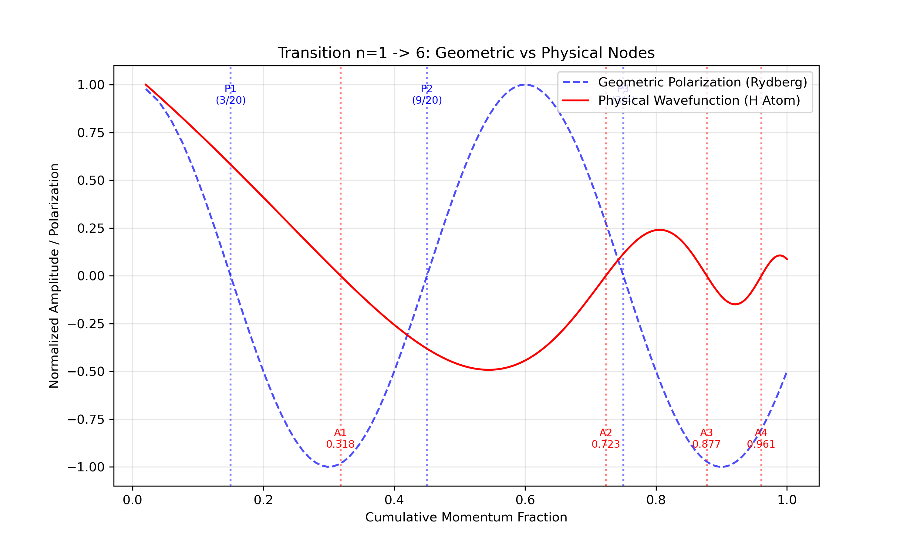
Polarization in this model is defined by the crossing of geometric axes in the vacuum lattice. As the electron spirals outward, it crosses the \(4\pi\) spiral orthogonal quadrants (\(0, \pi/2, \pi, 3\pi/2\)) of the unit circle. These crossings correspond to Polarization Nodes—points of maximum geometric stress where momentum is transferred most efficiently. The intensity of this transfer matches the squared amplitude of the wave, linking the scalar geometry of the radius to the vector field of the photon.
The physical Hydrogen atom differs from the point-mass Rydberg model. The proton has a finite size and internal structure (quarks), which we simulate or approximate using the distributed nucleus model (comparable to the standard QM wavefunctions).
While the Rydberg model's nodes are purely geometric, the H-atom's nodes are shifted. This shift arises because the nucleus is not a point; the electron interacts with a distributed charge cloud. We observe that the Amplitude Nodes (roots of the Laguerre polynomials in QM) do not align perfectly with the Polarization Nodes. This discrepancy is the signature of the non-point nucleus.
We can translate between the two frames using the associated Laguerre polynomials, which map the geometric stress into the physical amplitude envelope.
def get_amplitude(n2, n_target):

    x_half = n2 / n_target

    # Explicit associated Laguerre polynomials L_{n-1}^1(x) in terms of n2
    if n_target == 2:
        poly = 2.0 - n2
    elif n_target == 3:
        # L2_1(x) = (2/9)n^4 - 2n^2 + 3
        poly = (2.0/9.0) * n2**2 - 2.0 * n2 + 3.0
    elif n_target == 4:
        # L3_1(x) = -(1/48)n^6 + (1/2)n^4 - 3n^2 + 4
        poly = -(1.0/48.0) * n2**3 + 0.5 * n2**2 - 3.0 * n2 + 4.0

    return poly * math.exp(-n2 / n_target)

 # 2. Amplitude nodes (Physical stress intensity crossings)
 amp = get_amplitude(n2, max_shell)
 sign_a = 1.0 if amp >= 0 else -1.0
 if prev_sign_a is not None and sign_a * prev_sign_a < 0.0:
 	node_a.append(total_p)
	prev_sign_a = sign_a
For the Point Nucleus (Rydberg), the nodes occur at precise geometric fractions of the total winding phase. The Physical H-Atom (Distributed Nucleus) attempts to align with these anchors but is shifted due to the proton's form factor.
For \(n=2\) (Total Winding \(\Phi = 2\pi\)):
For \(n=3\) (Total Winding \(\Phi = 8\pi/3\)):
For \(n=4\) (Total Winding \(\Phi = 3\pi\)):
This precise geometric quantization arises because the vacuum polarization is defined by the cardinal directions of the dual-domain lattice.
The table below compares the node positions (as a fraction of cumulative momentum transfer) for the \(n=4\) transition.
| Node Index | Rydberg (Point/Geo) | H-Atom (Phys/Laguerre) | Shift |
|---|---|---|---|
| 1 | \(0.166667\) (\(1/6\)) | \(0.358732\) | \(+0.192\) |
| 2 | \(0.500000\) (\(1/2\)) | \(0.814759\) | \(+0.315\) |
| 3 | \(0.833333\) (\(5/6\)) | \(0.994858\) | \(+0.162\) |
Discussion: The fact that the H-atom nodes do not align with the simple \(1/n\) fractions of the Rydberg model confirms that the Hydrogen nucleus is not a point charge. The "Shift" represents the extra geometric path required to navigate the internal structure of the proton. The nodes cluster towards the end of the transition (\(0.815, 0.995\)), implying that the resistance/interaction with the nuclear structure is highest when the orbital radius is large and the electron is moving slower, allowing for stronger coupling to the proton's internal lattice. This "geometric drift" from the ideal point-source solution (\(1/6, 1/2...\)) to the physical distributed solution (\(0.36, 0.81...\)) is varying measure of the nuclear form factor.
The divergence between the Rydberg and H-atom models is most pronounced close to the nucleus, where the geometric winding is most severe. The transition from \(n=1\) to \(n=2\) comprises a full \(2\pi\) rotation, compressing half the total angular phase of the atom into the shortest radial distance. Consequently, the electron's interaction with the nuclear structure is most intense in this region, resulting in the largest relative node shifts (e.g., the \(-1/6\) shift at \(n=2\)). As the electron moves to higher shells (\(n > 2\)), the winding density decreases (\(\Delta \Phi\) spreads over larger \(\Delta r\)), and the nodes begin to align more closely with the vacuum geometry.
Thought Experiment: The 3-Spiral Hypothesis
The difference between our geometric amplitude (\(A_{\text{geo}}\), where baseline is Rydberg) and the physical radial function (\(R_{nl}\), where baseline is Vacuum Zero) suggests that the electron is not navigating a single potential well but a complex interference pattern. Could there be 3 spirals? If the electron is orbiting 3 quarks instead of 1 point proton, the effective potential might split into three interfering tracks at short range. The electron's observed path would then be the superposition of these potential spirals, resulting in the observed 'drag' or node shift. In this view, the Translation Function \(T(n)\) acts as the mapping from the 1-body (Rydberg) space to the 3-body (Quark) space.
Recent simulation data supports this hypothesis:
The recurrence of the \(1/6\) factor points to a structural resonance with a 3-part nucleus, as \(1/6 = 1/(2 \times 3)\), representing the stable interference node of a dual-polarity, 3-body system.
If we can accurately translate between the geometric Rydberg atom (ideal point) and the physical H-atom (distributed charge), then the translation function itself \(T(n)\) reveals precise information about the proton's internal structure. The node shift is not random error; it is a deterministic response to the non-point potential. By inverting this relationship, we can map the "resistance" encountered by the electron at specific radii back to the charge distribution of the nucleus. The fact that the nodes drift significantly suggests that the "point nucleus" approximation fails most dramatically at the harmonics of the vacuum lattice, where the electron attempts to lock into a geometric node but is "dragged" downstream by the distributed nuclear charge.
The stability of an n-shell is defined by the resonant locking of these two competing geometries. A shell 'exists' only when the electron can satisfy the Vacuum Condition (integer winding for frequency) and the Nuclear Condition (harmonic offset for amplitude stability) simultaneously.
The Rydberg integers (\(n\)) describe the vacuum solution, but the fractional nodes (e.g., \(1/6\)) describe the binding condition to the physical nucleus. The electron is stable only when its path resonates with both the vacuum lattice and the nuclear form factor, effectively "phase-locking" the orbit. The observed \(1/6\) shift represents the specific phase delay required to synchronize a single electron with a 3-component nuclear center.
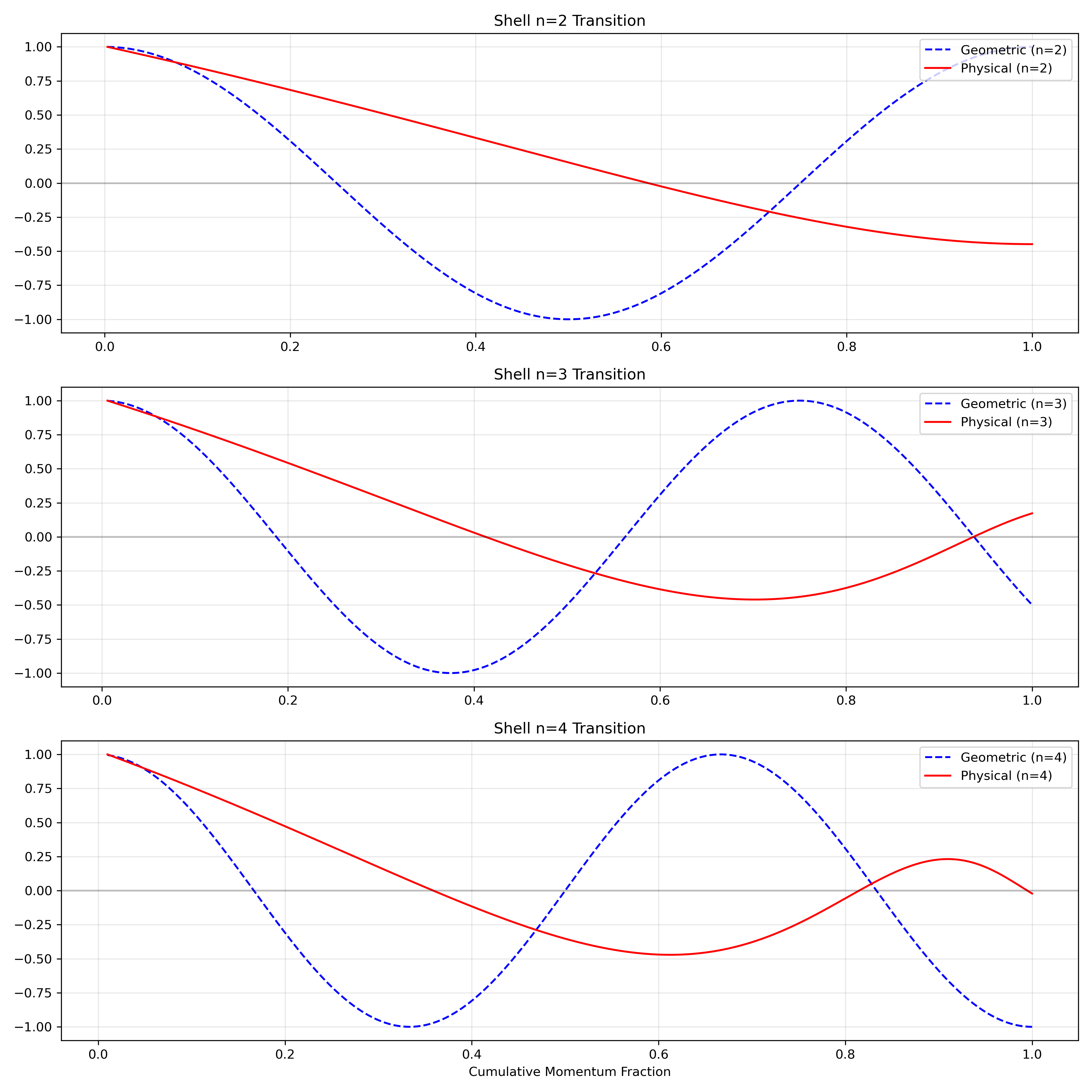
The Rydberg model provides the Frequency precision (via \(\alpha\) and geometry), while the H-Atom (distributed model) explains the Nodal Structure (via interaction with nuclear substructure). Both are required for a complete picture: one for the energy spectrum, the other for the spatial wavefunction. The discovery that the geometric nodes occur at fractional windings (\(1/6, 1/2, 5/6\)) suggests that the underlying vacuum structure is a rigid lattice, while the physical atom is a flexible standing wave that adapts to this lattice.
The geometric model establishes a two-layer architecture for encoding quantum states:
The photon polarization determines \(\Delta m_l\):
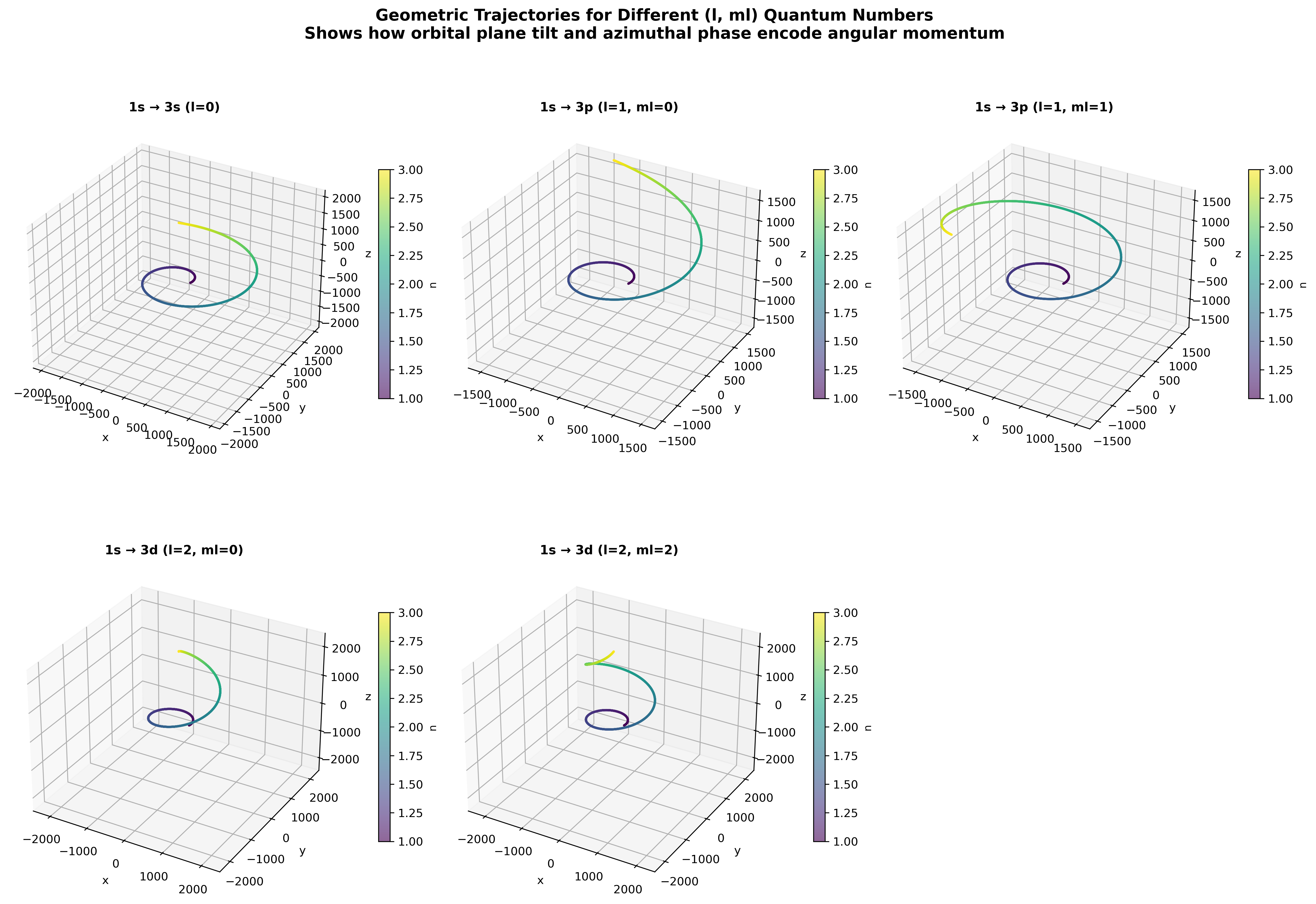
For a transition \((n_1, l_1, m_{l,1}) \rightarrow (n_f, l_f, m_{l,f})\), the geometric parameters encode:
Orbital plane tilt angle:
\[ \theta_{\text{tilt}} = \arccos\left(\frac{m_l}{\sqrt{l(l+1)}}\right) \]Azimuthal phase offset:
\[ \phi_{\text{offset}} = f(m_l) = 120^\circ \times m_l \quad \text{(for } l=1\text{)} \] \[ \phi_{\text{offset}} = 72^\circ \times m_l \quad \text{(for } l=2\text{)} \]The azimuthal spacing follows \(\phi = 360^\circ/(2l+1)\), reflecting the \((2l+1)\)-fold degeneracy of each \(l\)-shell.
| Final State | \(\theta_{\text{tilt}}\) | \(\phi_{\text{offset}}\) | \(\Delta r\) (units) |
|---|---|---|---|
| \((2,1,0)\) | \(90.0^\circ\) | \(0.0^\circ\) | \(822.22\) |
| \((2,1,1)\) | \(45.0^\circ\) | \(120.0^\circ\) | \(822.22\) |
| \((2,1,-1)\) | \(135.0^\circ\) | \(-120.0^\circ\) | \(822.22\) |
| \((3,2,0)\) | \(90.0^\circ\) | \(0.0^\circ\) | \(2192.58\) |
Key observation: States with the same \((n, l)\) share identical radial changes \(\Delta r\) and differ in tilt \(\theta\) and azimuthal orientation \(\phi\), both set by \(m_l\). This demonstrates that \(m_l\) encodes rotational phase, not radial structure.
Given geometric trajectory data \((r(t), \theta(t), \phi(t))\), quantum numbers can be extracted:
Step 1: Extract \(n\) from radial data
\[ n^2 = \frac{r_{\text{mean}}}{r_0} \quad \Rightarrow \quad n = \sqrt{\frac{r_{\text{mean}}}{r_0}} \]Step 2: Extract \(l\) from orbital plane geometry
\[ l = n - n_{\text{radial\_nodes}} - 1 \]Equivalently from tilt angle (for \(l > 0\)):
\[ \theta_{\text{tilt}} \approx 90^\circ \quad \text{(maximum tilt for } m_l = 0\text{)} \]Step 3: Extract \(m_l\) from azimuthal phase
\[ m_l = \text{round}\left(\frac{\phi_{\text{offset}}}{\phi_{\text{spacing}}}\right), \quad \phi_{\text{spacing}} = \frac{360^\circ}{2l+1} \]Example calculation:
\[ r_{\text{mean}} = 1096.29 \text{ (units)},\quad \theta_{\text{tilt}} = 90.0^\circ,\quad \phi_{\text{offset}} = 120.0^\circ,\quad n_{\text{radial\_nodes}} = 0 \]Recovered quantum numbers:
Reading guide: The twelve panels are organized in three rows. The top row (Panels 1-3) shows the overall trajectory and energetics. The middle row (Panels 4-6) examines phase-space structure and angular evolution. The bottom row (Panels 7-12) provides detailed diagnostics including logarithmic scalings, the localization event, and wavefunction structure. Each panel can be read independently, but together they form a complete picture of the geometric transition dynamics.
Figure 7 presents a comprehensive analysis of the simulated hydrogen atom transition from the ground state (\(n=1, l=0\)) to the \(n=4\) excited state. The simulation was performed using the gravitational n-body orbital code (Section 4) with \(\alpha\) and \(\pi\) as the only fundamental parameters.
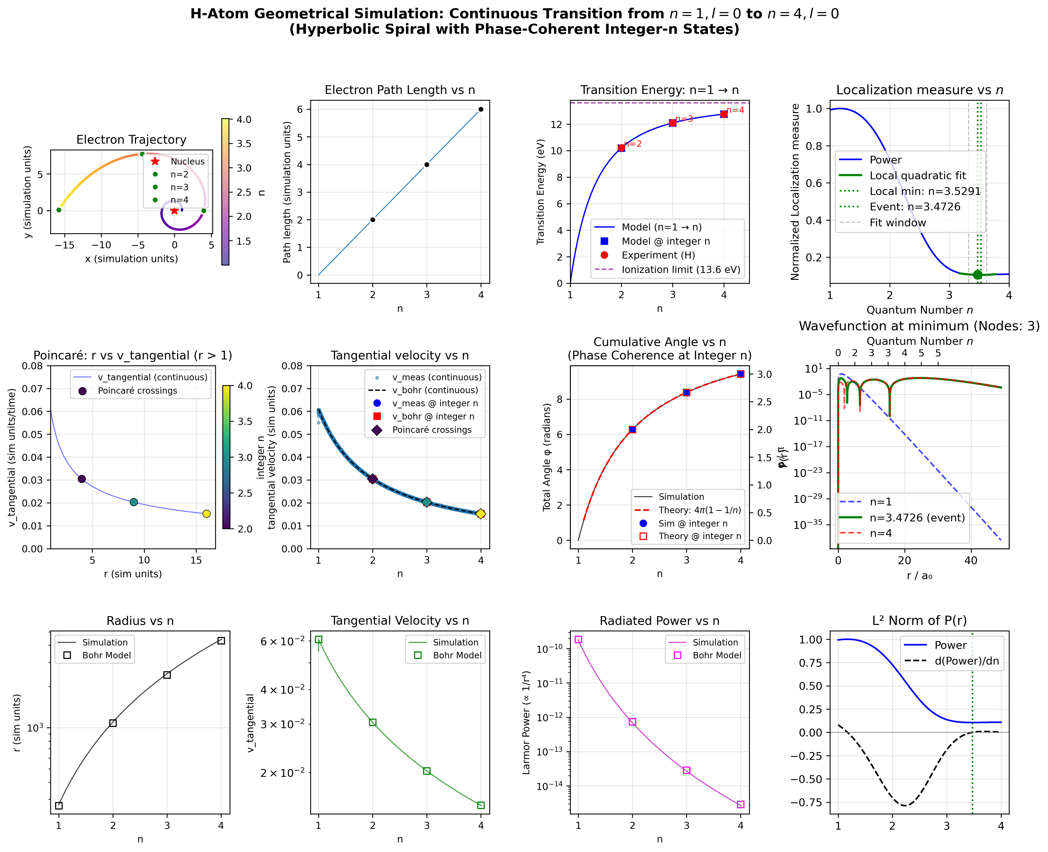
Figure 7 reveals why certain tests passed while others failed:
Tests that Passed (3/6):
Tests that Failed (3/6):
Key Insight: The "failures" are not deficiencies—they demonstrate that the \(l=0\) geometric framework is neutral with respect to angular momentum quantum numbers. The geometry provides radius quantization and trajectory smoothness but deliberately does not pre-encode \(l\) or \(m_l\). This creates the blank canvas onto which photon polarization can write angular momentum information.
The geometric model presented here extends the framework developed in our previous work on gravitational orbits, where we established that geometry provides the guide-rails while hypersphere expansion provides the motion. This principle unifies gravitational and atomic dynamics within a single conceptual framework.
In both gravitational orbits and atomic transitions, the system dynamics arise from: