
We present a geometric model of orbital mechanics in which gravitational and atomic orbits emerge from time-averaged networks of rotating point-to-point orbital pairs. The model discretizes macroscopic objects into Planck-mass points, each forming independent orbital pairs with all other points in the system, creating a universe-wide N-body network. Despite using only dimensionless rotating circles governed by the fine structure constant α and π, the model reproduces Kepler's law and anomalous orbital precession. The model operates at the Planck scale, with each orbital rotating through one Planck length per Planck time (velocity c in hypersphere coordinates). Crucially, the model treats particles as oscillations between an electric wave-state (duration: particle frequency) and a mass-point state (duration: one Planck time), thereby replacing 2 abstract forces with 2 distinct states through temporal averaging. We demonstrate that when the gravitational coupling constant αG is inverted, gravity becomes the dominant force at unit (Planck) time, with its apparent macroscopic weakness arising statistically from the rarity of mass-point states. The model uses only geometry, α, π, and Planck units for dimensional conversion.
Keywords: gravitational orbits, N-body simulation, Planck scale, fine structure constant, orbital precession, Kepler's laws, geometric quantization
The laws of orbital mechanics, from Kepler's empirical observations to Einstein's general relativistic corrections, describe what celestial bodies do but not fundamentally why they follow these patterns. Similarly, atomic orbitals are described by the Schrodinger equation's solutions, yet the physical mechanism underlying electron confinement remains interpretational rather than mechanical.
This work and the article on atomic orbitals [4] together propose a unified geometric framework wherein both gravitational and atomic orbits emerge from identical underlying dynamics: discrete rotations of orbital pairs at the Planck scale. The key innovation is treating macroscopic objects not as continuous entities but as collections of Planck-mass points (mP), each independently orbiting every other point in the universe.
The observed macroscopic orbits are emergent phenomena—statistical averages over vast numbers of microscopic orbital pairs.
Discrete particles in this model are replaced by a continuous electric wave-state to mass point-state oscillation.
Electric wave-state: Duration = particle frequency (measured in Planck time units). Position undefined; particle exists as extended wave.
Mass point-state: Duration = one Planck time tp. Position can be defined as a point.
The final particle frequency fparticle = (wave-state frequency + 1) tp.
This is a constant repeating oscillation and not a duality, the particle therefore exists over time and not at unit time, and so quantum theories cannot be applied to the Planck scale as baryonic matter does not exist as we know it at the Planck scale. Each electron oscillation cycle lasts 1023 units of Planck time (since electron frequency = mP/me = 1023 tp). As there are approximately 1043 units of Planck time in 1 second, this gives approximately 1020 oscillations per second. This artifice is also used to map atomic orbital transitions using a gravitational orbit simulator [4] as we now have 2 distinct particle states (wave and point) instead of 2 abstract forces (gravitational and electromagnetic).
Mass is not thus a constant property of particles, rather observed mass mobs is the frequency of occurrence of Planck mass units (mP). If the particle wave-state energy can be represented by E = hf and the mass state by E = mc2, and as for each wave-state there is a corresponding mass state (as the particle oscillates between both states) then we have an equivalence between hf and mobsc2. Both h and c are fixed constants, and so f and mobs are the frequency components; f measures the frequency of occurrence of a unit of h per second and the mobs term measures the frequency of occurrence of a unit of mP per second (if there are 10 wave-states per second then there are also 10 mass states per second).
Note (Domain Link): The mass point-state corresponds to the Matter (Integer) Domain where the particle has defined position and mass. The electric wave-state corresponds to the Radiation (√Integer) Domain where the particle exists as an extended wave. This oscillation between domains underlies wave-particle duality.
As gravitational orbits only emerge over time from the sum of these orbital rotations occurring at unit time, it is helpful to run simulations to measure the outcome. These orbitals can be simulated on a 2-D plane representing 3-D space. Macro-objects A, B, C .... are divided into points, each point assigned initial Cartesian co-ordinates (x, y), and these points then form orbital pairs with all other points. The barycenter for each orbital pairing is its orbital center, the points located at each orbital 'pole'.
The simulation increments in integer steps (each step equates to 1 unit of time), during each step, the orbitals rotate 1 unit of length. Each orbital is calculated independently of all other orbitals, for the simulation there are no macro-objects A, B, C... (there are only discrete orbitals), however the initial (x, y) point co-ordinates will reflect the spatial co-ordinates of these macro-objects.
These rotations at unit time are then summed and averaged to give new co-ordinates, the process repeated and the results then mapped over time to reflect the orbits. The programs used to simulate the orbits can be accessed here [code repository].
Modelling (simulating) gravitational effects at the macro scale requires objects to have (for each unit of Planck time) a minimum mass >= Planck mass (minimum = 1 mass point). This is because whilst in this mass point-state, a particle can be assigned mapping coordinates. For example, an electron has a frequency = 1023tp and so an electron would have (would be) mass only once every 1023 units of Planck time. If a (hypothetical) object composed only of electrons is to have constant mass (to have 1 unit of Planck mass at every unit of Planck time), then that object will require 1023 electrons, such that on average there will always be 1 electron in the mass point-state. A 1kg satellite would have 1kg/mP = 45940509 mass points (45940509 of its particles in the mass state) at any 1 unit of Planck time (although at each unit of time different particles would be in the point state as they oscillate). During the wave-state the particle has no fixed co-ordinates (and so in atomic orbital simulations it is represented by a wave-function or probability density).
We can then divide orbiting objects A, B, C... into discrete (Planck mass) points, each point = 1mP. Each point in object A then forms an orbital pair with every point in objects B, C..., resulting in a universe-wide, n-body network of rotating point-to-point orbital pairs (3 points = 3 orbitals, 4 points = 6 orbitals, 8 points = 28 orbitals ...).
The clock-rate of the simulation can be expressed as a programming loop;
FOR tage = 1 (big bang) TO (the end)
rotate all orbital pairs
sum and average new positions
assign new co-ordinates to the points
NEXT
After each increment to the clock-rate (1 unit of simulation time), all orbitals rotate 1 unit of length, the results are then summed and averaged, and the new co-ordinates assigned to the points.
The model itself is dimensionless, to convert to real world orbits the Planck units can be used; 1 unit of mass == Planck mass mP, 1 unit of time == Planck time tp and 1 unit of length == Planck length lp. This would translate to 2 Planck mass points (2 points per orbital) travelling 1 unit Planck length per unit of Planck time (which is velocity c = lp / tp) in hypersphere coordinates (3-D space is seen as the surface of a 4-axis expanding hypersphere) [2].
2-body orbits comprise a radius constant \({1/\alpha}\) (the fine structure constant alpha) and a radius wavelength.
\[ {r_{\alpha}}^2 = \frac{2}{\alpha} = 274.071998354 \]The radius wavelength rwavelength defines orbital radius in terms of the central mass and the orbiting point, thus quantizing the radius.
\[ r_{orbit} = {r_{\alpha}}^2\; *\; r_{wavelength} \]The central mass Schwarzschild radius = i and the total mass = j. This \({r_{orbital}}^{-3/2}\) dependence is fundamental to the model as it determines the velocity of the orbit on a 2-D plane (representing 3-D space). Note, in hypersphere co-ordinates orbital velocity occurs at c but this article is principally concerned with orbits in 3-D space.
\[ \beta_{orbital} = \frac{1}{r_{ij} r_{orbital} \sqrt{r_{orbital}}} \] \[ r_{ij} = \sqrt{\frac{2 j}{i}} \]For simple 2-body orbits, to reduce computation 1 point is assigned as the orbiting point and the remaining points are assigned as the central mass. For example the ratio of earth mass to moon mass is 81:1, and so we could simulate this orbit accordingly with 82 points by assigning (x, y) co-ordinates for 81 points in close vicinity (the central mass) and 1 point with co-ordinates at distance from the center (the orbiting mass). However we note that the only actual distinction between a 2-body orbit and a complex multi-body orbit being that the central mass points are assigned co-ordinates relatively close to each other, and the orbiting point is assigned co-ordinates at distance (this becomes the orbital radius) ... this is because the simulation treats all points equally, the center points also orbiting each other according to their orbital radius, for the simulation itself there is no distinction between simple 2-body and complex n-body orbits.
The Schwarzschild radius formula in Planck units
\[ r_s = \frac{2 l_p M}{m_P} \]As the simulation itself is dimensionless (merely rotating orbitals on a 2-D plane), we can remove the dimensioned Planck length component \(2 l_p\), and as M is divided into discrete Planck mass units, the Schwarzschild radius for the simulation can then be reduced to the number of central mass points
\[ i = \frac{M}{m_P} \]We then assign (x, y) co-ordinates (to the central mass points) to represent the spatial dimensions of this central mass.
Note (Atomic-Gravitational Parallel): The orbital radius formula \(r_{orbit} = \frac{2}{\alpha} \times r_{wavelength}\) has the same structure as the atomic Bohr radius: \(a_0 = \frac{2}{\alpha} \times \lambda_{Compton}\). In atomic orbitals the wavelength is the Compton wavelength; in gravitational orbitals it is the Schwarzschild radius. The fine structure constant α appears in both as the sole fundamental coupling constant.
Running this 11-body orbit simulation gave [nbody code];
orbit period = 1076159500
orbit length = 1818510.979169879
orbit barycenter; x = 28942.502425, y = 0.001086
From these simulation results the following formulas were derived.
radius of orbiting point (from center)
\[ r_{orbit} = {r_{\alpha}}^2\; 2 \frac{(k_r i + 1)^2}{i^2} \]velocity of orbiting point
\[ v_{orbit} = \sqrt{\frac{i}{r_{orbit} j}} \]reduced mass (orbit occurs around the barycenter)
\[ \mu = \frac{i \times 1}{i + 1} = \frac{i}{i + 1} \]orbiting point period
\[ t_{orbit} = 2\pi \mu \frac{r_{orbit}}{v_{orbit}} = 2\pi \frac{8} {{\alpha}^{3/2}} \frac{{(k_r i + 1)}^3}{i^{5/2} j^{1/2}} \]barycenter
\[ r_{barycenter} = \frac{r_{orbit}}{j} \]length of orbit
\[ l_{orbit} = 2 \pi (r_{orbit} - r_{barycenter}) \]Solving these equations using the above parameters (i = 10, j = 11, kr = 24)
Calculated (orbital formulas):
orbit period = 1076159506.7957308
orbit radius = 318367.514728
orbit length = 1818510.9916564
orbit barycenter = 28942.5013389, 0
Significance: The simulation results verify that orbit like conditions can be achieved using rotating orbitals and that this set of formulas can accurately reflect those orbits. The next step is to demonstrate that these formulas can also be applied to real-world orbits, and thereby confirm that this rotating orbital model can in fact replicate gravitational orbits.
The earth to moon mass ratio approximates 81:1 and so can be simulated as a 2-body orbit with the moon as a single orbiting point as in the above example. Here we use the orbital parameters to determine the value for the mass to radius coefficient kr. (note: here are used Planck length lp, Planck mass mP and c to convert between the dimensionless simulation and dimensioned SI units).
Reference values
M = 5.9722 × 1024kg (earth)
m = 7.346 × 10²²kg (moon)
To = 27.321661 × 86400 = 2360591.51s
To simplify, we assume a circular orbit which gives this radius
\[ R_o = \left(\frac{G (M+m) T_o^2}{4 \pi^2}\right)^{(1/3)} \]Ro = 384714027m
G = 0.66725e-10
The mass ratio i = 81.298666, j = i + 1
\[ i = \frac{M}{m} \]We then find a value for kr using To as our reference (reversing the orbit period equation).
\[ t_{orbit} = 2\pi \frac{8} {{\alpha}^{3/2}} \frac{{(k_r i + 1)}^3}{i^{5/2} j^{1/2}} \] \[ k_r = \frac{1}{i} {\left(\frac{t_{orbit} i^{5/2} j^{1/2}{\alpha}^{3/2}}{16 \pi }\right)}^{(1/3)} - \frac{1}{i} \] In dimensioned terms (Planck units) \[ T_o = t_{orbit} \frac{l_p}{c} \frac{M}{m_P} \] And so we can numerically solve torbit and thenkr = 12581.4468
We then use the 2-body orbit formulas to solve these parameters (dimensionless)
rorbit = 86767420100
torbit = 0.159610040233 × 10¹⁸
rbarycenter = 1054299229.62
lorbit = 538551421685
vorbit = 0.33741701 × 10⁵
Converting back to dimensioned values
\[ R_o = r_{orbit} l_p \frac{M}{m_P} \] \[ T_o = t_{orbit} \frac{l_p}{c} \frac{M}{m_P} \]R = 384714027m = Ro
T = 2360591.51s = To (used to align kr with the earth-moon orbit)
B = 4674608.301m (barycenter)
L = 2387858091.51m (distance travelled by the moon)
V = 1011.551m/s (velocity of the moon around the barycenter)
If we expand the velocity term
\[ v_{orbit} = \sqrt{\frac{i}{r_{orbit}j}} \] \[ v_{orbit}^3 = \frac{G M}{T_{orbit}} 2\pi \frac{i^2}{j^2} \]Kepler's formula reduces to G
\[ R = \frac{2}{\alpha}\; 2 \frac{(k_r i + 1)^2}{i^2} l_p \frac{M}{m_P} \] \[ T = \frac{16 \pi} {{\alpha}^{3/2}} \frac{{(k_r i + 1)}^3}{i^{5/2}(i+1)^{1/2}} \frac{l_p}{c} \frac{M}{m_P} \] \[ M+m = M \left(\frac{i+1}{i}\right) \] \[ \frac{4 \pi^2 R^3}{(M+m) T^2} = \frac{l_p c^2}{m_P} = G \]# Maple code R:=(2/alpha)*2*((kr*i+1)^2/i^2)*lp*(M/mP): T:=(16*Pi/alpha^(3/2))*((kr*i+1)^3/(i^(5/2)*(i+1)^(1/2)))*(lp/c)*(M/mP): Mm:=M*(i+1)/i: simplify(4*Pi^2*R^3/(Mm*T^2)); # Output: lp*c^2/mP
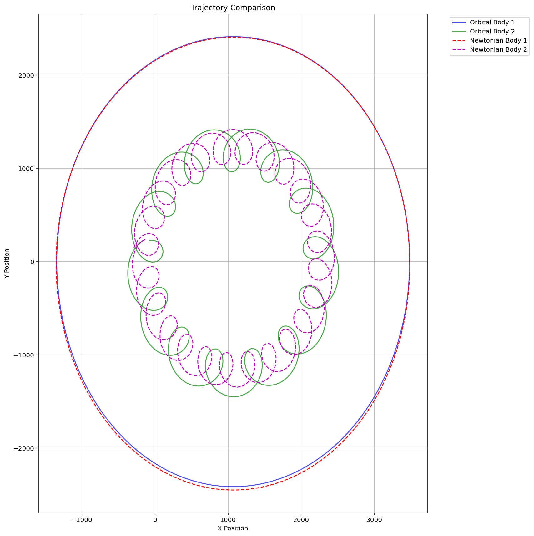
Orbital trajectory is a measure of alignment of the orbitals. In the above examples, all orbitals rotate in the same direction = aligned. If all orbitals are unaligned the object will appear to 'fall' = straight line orbit.
In this example (fig.1), for comparison, onto an 8-body orbit (blue circle orbiting the purple center mass), is imposed a single point (yellow dot) with a ratio of 1 orbital (anti-clockwise around the center mass) to 2 orbitals (clockwise around the center mass) giving an elliptical orbit.
The change in orbit velocity (acceleration towards the center and deceleration from the center) derives automatically from the change in the orbital radius, the only additional information is the orbital rotation direction.
An orbital drift (as determined where the blue and yellow meet) naturally occurs; the eccentricity (shape) of the orbit a function of center mass and the ratio of alignment of the orbitals. A near straight line orbit will have a greater drift and a greater eccentricity than a near circular orbit. The elliptical orbit has a longer period than the circular orbit (which has a 360 degree orbit, the sidereal period). The additional period is known as the anomalistic period and includes the precession angle (360 + precession angle). Note: in these simulations there are only 2 orbital types; clock-wise and anti-clockwise ... in a real world orbit there will be a complex mixture.

In classical mechanics, systems evolve along paths that minimize the action integral \(S = \int (KE - PE) \, dt\). In this model, the principle of least action emerges organically from geometric averaging.
Mechanism: Consider a 1kg satellite orbiting Earth. At any unit of Planck time, approximately 1040 distinct orbital pairs are active. Each orbital pair rotates independently, contributing to the satellite's trajectory.
Key insight: The satellite, through its constituent particles, is simultaneously following every possible path—each orbital pair represents one trajectory component. The observed macroscopic path is the statistical average of all these paths.
The path of minimum action corresponds to the configuration where orbital alignment (GKE) and misalignment (GPE) balance optimally. This is not imposed as a constraint but emerges from the averaging process over ~1040 orbitals.
Implication: The variational principles of classical and quantum mechanics (Lagrangian, Hamiltonian, Feynman path integral) can be understood as emergent statistical properties of this underlying geometry.
Precession is a change in the orientation of the rotational axis of a rotating body. The first of three tests to establish observational evidence for the theory of general relativity, as proposed by Albert Einstein in 1915, concerned the "anomalous" precession of the perihelion of Mercury. This precession is not predicted by Newtonian gravity.
The formula for precession uses the semi-major axis a and the semi-minor axis b.
\[ e = \sqrt{1-\frac{b^2}{a^2}} \] \[ \theta = \frac{6\pi G M}{a (1-e^2) c^2} \]Where e is the eccentricity of the orbit and θ is the precession angle.
As the frequency of the center mass Schwarschild radius = \(i 2 l_p\), and as i is the number of Planck mass points in the center mass and lp is Planck length; a and b become
\[ a = r_a i 2 l_p \] \[ b = r_b i 2 l_p \]The Schwarzschild radius of the sun λsun = 2953.25m. The eccentricity of Mercury e = 0.2056 (where a = 57909050km and b = 56671523km). From observational data, Mercury's perihelion advances by 43.1 arcseconds per century (after removing planetary perturbations).
\[ \theta_{\text{GR}} = \frac{6\pi GM_{\odot}}{ac^2(1-e^2)} = \frac{6\pi \lambda_{\text{sun}}}{2a(1-e^2)} \] \[ \theta_{\text{GR}} = \frac{6\pi \times 2{,}953}{2 \times 5.791 \times 10^{10} \times (1-0.2056^2)} = 0.501866 \times 10^{-5}\,\text{rad} \]Because the simulation is dimensionless, it can be mapped back to Standard International (SI) units or physical quantities by assigning each discrete orbital point a mass of one Planck mass (mP). By defining the central cluster as M points (M mP) and the orbiting body as a single point (\(1 m_P\)), the simulation metrics can be directly evaluated against classical physics expectations.
When comparing the simulated N-body precession against the continuous GR prediction, a profound relationship emerges depending on the ratio of the central mass to the orbiting mass (M/m).
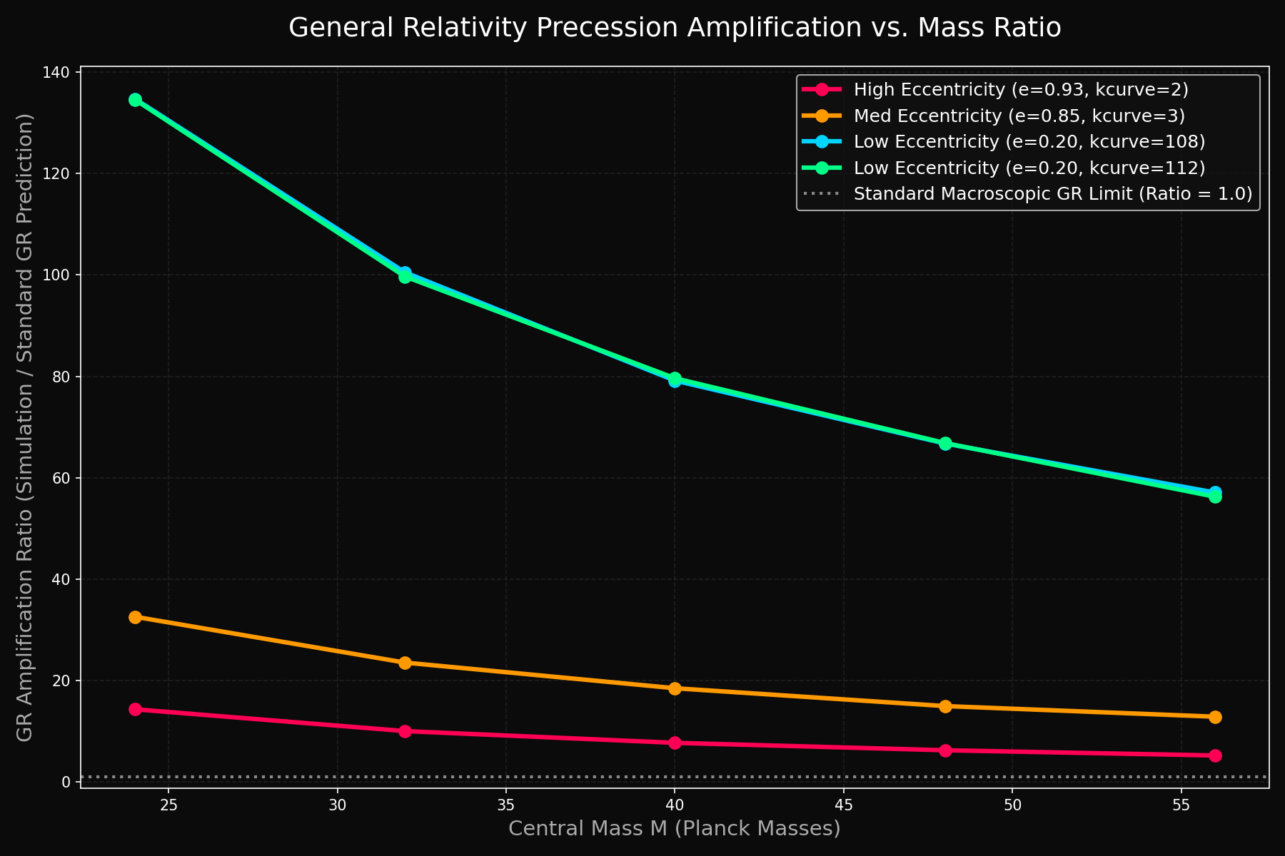
As shown in Figure 2, at small mass ratios (e.g., M = 24mP), the simulation produces a periapsis precession vastly larger than what standard isolated two-body General Relativity predicts. We term this phenomenon discrete frame-dragging. Because the central mass M is composed of discrete points (each also orbiting each other as an n-body orbit), the gravitational pull from the orbiting body m causes the internal structure of the core to "slosh" or physically displace in a rhythmic wobble (barycenter displacement). This violent internal core movement heavily warps the local orbital frame, dragging the reference particle and inducing a significantly amplified precession.
However, as the central mass integer grows (M ≫ m), the internal rigidity of the barycenter increases, and the amplification factor drops asymptotically toward 1.0. This demonstrates that at macroscopic, cosmic scales, the localized discrete frame-dragging diminishes, and the quantized simulation naturally converges back to continuous General Relativity predictions.
To allow for independent confirmation of these findings, the raw data comparing the simulated precession against the expected macroscopic GR prediction for four different eccentricity profiles (e) is provided in Table 1. These 4 data sets are from a clockwise-anticlockwise orbital ratio kcurve: 112:1, 108:1, 3:1, 2:1
| Central Mass (M) | e ≈ 0.93 | e ≈ 0.85 | e ≈ 0.20 (Curve A) | e ≈ 0.20 (Curve B) |
|---|---|---|---|---|
| 24 mP | 14.32 | 32.58 | 134.73 | 134.59 |
| 32 mP | 10.02 | 23.53 | 100.51 | 99.70 |
| 40 mP | 7.71 | 18.48 | 79.16 | 79.63 |
| 48 mP | 6.24 | 14.95 | 66.75 | 66.85 |
| 56 mP | 5.21 | 12.86 | 57.09 | 56.25 |
| ... | ... | ... | ... | ... |
| ∞ | ≈ 1.00 | ≈ 1.00 | ≈ 1.00 | ≈ 1.00 |
Significance: Despite quantitative limitations, the key achievement is that orbital precession can emerge naturally from purely geometric principles:
In the above, particles were assigned a mass as a unit of Planck mass. Conventionally, the gravitational coupling constant αG characterizes the gravitational attraction between a given pair of elementary particles in terms of a particle (i.e.: electron) mass to Planck mass ratio;
\[ \alpha_G = \frac{G m_e^2}{\hbar c} = 1.75... \times10^{-45} \]In the simulation, particles are treated as an oscillation between an electric wave-state (duration particle frequency) and a mass point-state (duration 1 unit of Planck time). This αG then represents the probability that any 2 specific electrons will be in the mass point-state at the same unit of Planck time = \((\frac{m_e}{m_P})^2\).
\[ \alpha_G = \frac{G m_e^2}{\hbar c} = \left(\frac{m_e}{m_P}\right)* \left(\frac{m_e}{m_P}\right) = 1.75... \times10^{-45} \]As 1 second requires 1043 units of Planck time, this will occur about once every 2-3 minutes and so gravity's apparent weakness is simply because the mass-state occurs so seldom relative to the particle wave-state.
We can define the coupling between any 2 objects; for a 1kg satellite orbiting the earth, for any unit of time the satellite (A) will have 1kg/mP = 45.9 ×10⁶ particles in the point-state. The earth (B) will have 5.97 ×1024 kg/mP = 0.274 ×1033 particles in the point-state, and so the number of links (rotating orbital pairs for any unit time) between the earth and the satellite will sum to;
\[ N_{orbitals} = \frac{m_A m_B}{m_P^2} = 0.126\; \times10^{41} \]With each increment to the simulation clock, the rotating orbital pairs will change as different particles enter/leave the mass-point state, nevertheless the average number of mass points per unit time remains the same.
Earth parameters: (mass = 5.9722e24kg)
\[ i = \frac{M_{earth}}{m_P} = 0.274366 \;\times10^{33} \] \[ i 2 l_p = 0.00887m \;(Schwarzschild \;radius) \] \[ s = \frac{1kg}{m_P} = 45940509 \] \[ N_{orbitals} = i*s = 0.126045 \;\times10^{41} \]In the 2-photon model [4], (mathematically) we separate the incoming photon into 2 photons (initial and final) as per the Rydberg formula.
\[ \lambda_{photon} = R\;\left(\frac{1}{n_i^2}-\frac{1}{n_f^2}\right) = \frac{R}{n_i^2}-\frac{R}{n_f^2} \] \[ \lambda_{photon} = (\lambda_i) - (\lambda_f) \]\((\lambda_i)\) is equivalent to the existing orbital and \((\lambda_f)\) is equivalent to the final orbital and so we are changing 1 orbital for another orbital. We can use the same model here.
Gravitational Rydberg
\[ r_{orbit} = \frac{2}{\alpha}\; *\; r_{wavelength} \] \[ E_{\text{orbital}} = \frac{hc}{2\pi r_{orbit}} \]Separating the fixed constants from the variable (the radius `wavelength component')
\[ R_g = \frac{hc \alpha}{4\pi} \]Example: Energy Requirements to lift a 1 kg satellite from Earth's surface to geosynchronous orbit (R = 42,164 km). We can calculate the wavelength part of each orbit;
\(r_{6731} = 6371000 \times \frac{2}{\alpha}\)
\(r_{42164} = 42164000 \times \frac{2}{\alpha}\)
Per orbital pair:
\[ E_{\text{orbital}} = R_g \left(\frac{1}{r_{6731}} - \frac{1}{r_{42164}}\right) = 4.21255 \times 10^{-33}\,\text{J} \]Number of orbital pairs:
\[ N_{\text{pairs}} = \frac{M_{\text{Earth}} \cdot 1\,\text{kg}}{m_P^2} = 1.26045 \times 10^{41} \]Total energy:
\[ E_{\text{total}} = E_{\text{orbital}} \times N_{\text{pairs}} = 5.3097 \times 10^{7}\,\text{J} = 53.1\,\text{MJ/kg} \]This closely matches the actual Δv energy requirement for launch to geosynchronous orbit (~50–60 MJ/kg), validating the model's energy accounting. A full discussion of the 2-photon model is given in the article on atomic orbital transitions and so is not repeated here [4].
At any unit of Planck time, approximately 1060 orbital pairs are active. Over one second (~1043 Planck times), the total number of orbital-pair rotation events is:
\[ N_{\text{events}} = N_{\text{orbitals}} \times \frac{1\,\text{s}}{t_p} \approx 10^{103} \]This astronomical number explains why macroscopic gravity appears smooth and continuous—it's a statistical average over incomprehensibly many discrete events.
The orbital angular momentum of a planet can be calculated directly from the number of orbital pairs. For a planet of mass Mplanet orbiting the Sun (Msun = 1.988435 × 1030 kg):
\[ L = \frac{M_{sun}}{m_P} \cdot \frac{M_{planet}}{m_P} \cdot \frac{hc}{2\pi} = N_{orbitals} \cdot \hbar c \]This formula gives the angular momentum as a function of the number of orbital pairs. To compare with observed values, we divide by the orbital velocity to obtain L/v:
| Planet | Mass (kg) | Velocity (m/s) | Estimated | Calculated |
|---|---|---|---|---|
| Mercury | 3.302 × 10²³ | 47870 | 9.1 × 1038 | 9.15 × 1038 |
| Venus | 4.867 × 1024 | 35020 | 1.8 × 1040 | 1.84 × 1040 |
| Earth | 5.972 × 1024 | 29780 | 2.66 × 1040 | 2.66 × 1040 |
| Mars | 6.417 × 10²³ | 24130 | 3.52 × 1039 | 3.53 × 1039 |
| Saturn | 5.683 × 1026 | 9670 | 7.9 × 1042 | 7.80 × 1042 |
| Jupiter | 1.899 × 1027 | 13070 | 2.0 × 1043 | 1.93 × 1043 |
The close agreement between observed (estimated) angular momentum and the orbital-pair calculation demonstrates that planetary orbital dynamics can be derived directly from the number of Planck-scale rotating orbital pairs.
Significance: In standard cosmology, planetary orbital angular momentum is understood as inherited from the angular momentum of the primordial gas and dust cloud that formed the Solar System—a historical property. In this model, however, the angular momentum is a geometric consequence of the orbital pair structure: it is determined entirely by the masses involved, not by "remembering" initial conditions. The orbital pairs define the angular momentum; the history is irrelevant.
Key insights:
This resolves the "hierarchy problem" of why gravity is 1040 times weaker than electromagnetism: it's a consequence of temporal duty cycles, not coupling strengths.
The simulation itself does not distinguish between objects, its treats all points independently and so an orbit with 3 points is a 3-body orbit (3 orbitals), 26 points is a 26-body orbit (325 orbitals). In the 2 body examples above however we have placed most points in relatively close vicinity to simulate a center object around which a point then rotates. The resulting orbit derives from the start co-ordinates assigned to the points, assigning the points start co-ordinates via random numbers will result in a `dust' cloud orbit.
Examples:


The simulation embeds 3D space in a 4D hypersphere expanding at constant velocity [2]. Coordinates are:
Expansion rate:
\[ \frac{dR}{dt} = c = \frac{l_p}{t_p} \]All particles are "carried along" by this expansion. In the hypersphere reference frame:
\[ \vec{v}_{\text{total}}^2 = \vec{v}_{\text{spatial}}^2 + \vec{v}_{\text{expansion}}^2 = c^2 \]Therefore, if an object has spatial velocity v (e.g., orbiting), its expansion velocity is:
\[ v_{\text{expansion}} = \sqrt{c^2 - v^2} \approx c \left(1 - \frac{v^2}{2c^2}\right) \]This automatically produces time dilation—objects moving spatially experience slower expansion (aging) relative to stationary objects.
An object B orbiting object A traces a helical path in 4D:
From A's perspective:
This explains why orbital mechanics calculations use 3D spatial coordinates only—the z component is universal and cancels out in relative measurements.
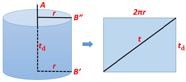
In (fig. 6), while B (satellite) has a circular orbit period on a 2-axis plane (horizontal axis as 3-D space) around A (planet), it also follows a cylindrical orbit (from B' to B'') around the A (vertical) time-line expansion axis. A moves with the universe expansion (along the time-line z axis) at (v = c) but is stationary in 3-D space (v = 0). B is orbiting A at (v = c) but the time-line axis motion is equivalent (and so `invisible') to both A and B, as a result the orbital period and velocity measures will be defined in terms of 3-D space co-ordinates by observers on A and B.
The hypersphere model bears formal resemblance to:
| Aspect | Newton | This Model |
|---|---|---|
| Force law | F = Gm1m2/r2 | No forces; rotating orbitals |
| Action-at-a-distance | Instantaneous | Mediated by point-pair rotations |
| Continuous trajectories | Yes | Emergent from discrete events |
| Kepler's laws | Derived from F=ma | Derived from geometric averaging |
| Precession | Requires perturbations | Emerges from orbital misalignment |
| Gravitational constant | Fundamental parameter | Derived: G = lp c2 / mP |
Agreement: Both reproduce Kepler's laws and two-body orbital mechanics to high precision.
Divergence: Newton treats gravity as an instantaneous force; our model treats it as a statistical average of local rotations propagating at c.
| Aspect | GR | This Model |
|---|---|---|
| Spacetime | Continuous manifold | Discrete network of events |
| Curvature | Riemann tensor | Orbital-pair interference |
| Geodesics | Extremal proper time | Averaged orbital paths |
| Perihelion precession | Schwarzschild metric | Geometric misalignment |
| Frame dragging | Kerr metric | Central mass rotation |
| Gravitational waves | Ripples in spacetime | (Not yet explored) |
| Planck scale | Breakdown scale | Fundamental scale |
[1] Macleod, Malcolm J. "The Programmer God, are we in a simulation?" theprogrammergod.com
[2] Macleod, M.J. Programming Planck units from a virtual electron: a simulation hypothesis. Eur. Phys. J. Plus 133, 278 (2018). https://doi.org/10.1140/epjp/i2018-12094-x
[3] Macleod, Malcolm J., 1. Planck unit scaffolding to Cosmic Microwave Background correlation https://www.doi.org/10.2139/ssrn.3333513
[4] Macleod, Malcolm J., 2. Relativity as the mathematics of perspective in a hyper-sphere universe https://www.doi.org/10.2139/ssrn.3334282
[5] Macleod, Malcolm J., 3. Gravitational orbits from n-body rotating particle-particle orbital pairs https://www.doi.org/10.2139/ssrn.3444571
[6] Macleod, Malcolm J., 4. Geometrical origins of quantization in H atom electron transitions https://www.doi.org/10.2139/ssrn.3703266
[7] Macleod, Malcolm J., 5. Atomic Transitions via a Photon-Orbital Hybrid https://www.doi.org/10.13140/RG.2.2.10680.20487
[8] Macleod, Malcolm J., 6. Do these anomalies in the physical constants constitute evidence of coding? https://www.doi.org/10.2139/ssrn.4346640
[9] Macleod, Malcolm J., 7. Geometric Origin of Quarks, the Mathematical Electron extended https://www.doi.org/10.13140/RG.2.2.21695.16808
[10] Macleod, Malcolm J., 8. Holographic Emergence in the Simulation Hypothesis https://www.doi.org/10.13140/RG.2.2.20919.28320