2. Relativity as the mathematics of perspective in a hyper-sphere universe

Introduction

This (mathematical universe [1]) model uses the Planck units to form the scaffolding for the particle universe. Instead of a dark energy, these units are added incrementally according to a defined geometrical framework thereby forcing the expansion of the universe in (Planck) units of mass, space and time [3]. In this article we compare the co-ordinate systems for this Planck unit lattice structure within an expanding 4-axis hyper-sphere reference with our 3-D space (as residing on the surface of the hyper-sphere).

Planck lattice

The sum universe expands incrementally. With each increment a set of Planck units are added (the method for adding the Planck units via dimensionless geometrical objects is described in the article on Planck unit anomalies [7], see also sect. 9). As for each unit of Planck time \(t_p\) added, there is also a corresponding unit of Planck length \(l_p\) added, and so this Planck lattice is expanding at a constant rate (the speed of light \(c = l_p / t_p\)). This forms a `Newtonian' background albeit the universe is constantly expanding in these discrete Planck unit steps at the speed of light.

Wave-particle oscillation

Discrete particles in this model are replaced by a continuous electric wave-state to mass point-state oscillation.

Electric wave-state: Duration = particle frequency (measured in Planck time units). Position undefined; particle exists as extended wave.

Mass point-state: Duration = one Planck time \(t_p\). Position can be defined as a point.

The final particle frequency \(f_{particle}\) = (wave-state frequency + 1) \(t_p\).

This is a constant repeating oscillation and not a duality, the particle therefore exists over time and not at unit time, and so quantum theories cannot be applied to the Planck scale as baryonic matter does not exist at the Planck scale. Each electron oscillation cycle lasts \(10^{23}\) units of Planck time (since electron frequency = \(m_P/m_e\) = \(10^{23} t_p\)). As there are approximately \(10^{43}\) units of Planck time in 1 second, this gives approximately \(10^{20}\) oscillations per second. This artifice is also used to map atomic orbital transitions using a gravitational orbit simulator [4] [5] as we now have 2 distinct particle states instead of 2 abstract forces.

Mass is thus not a constant property of particles, rather observed mass \(m_{obs}\) is the frequency of occurrence of Planck mass units (\(m_P\)). If the particle wave-state energy can be represented by \(E = hf\) and the mass state by \(E = mc^2\), and as for each wave-state there is a corresponding mass state (as the particle oscillates between both states) then we have an equivalence; \(hf = m_{obs}c^2\). Both \(h\) and \(c\) are fixed constants, and so \(f\) and \(m_{obs}\) are the frequency components; \(f\) measures the frequency of occurrence of \(h\) per second and the \(m_{obs}\) term measures the frequency of occurrence of \(m_P\) per second.

Space-time

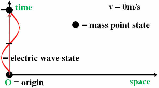
4.1. Particle A is mapped onto a space-time graph (fig.1). A does not move in space (\(v = 0\)), but it does move in time. The red sin wave represents the particle electric wave-state, the black dot as the mass point-state.

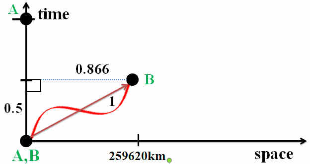
4.2. Particle B, \(v = 0.866c\) is added (fig.2). After 1s B will have traveled \(0.866 \times 299792458 = 259620\) km from A along the horizontal space axis. Particle B has the same wavelength as A (they are the same particle).

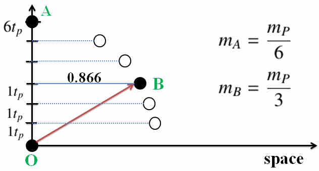
4.3. Particles A and B both have a frequency \(f = 6\); \(5t_p\) (5 units of Planck time) in the wave-state then \(1t_p\) (1 unit of Planck time) in the Planck mass point-state. As the A point-state occurs once every \(6t_p\), mass of A (\(m_A = m_P/6\)), however as we saw in fig. 2, particle B's time is running at 0.5× the speed of particle A's time. In its own reference frame, B still completes 6 oscillations, but from A's perspective, these 6 oscillations are compressed into only 3 units of A's time (\(6 \times 0.5 = 3\)). Because mass is measured by the frequency of these oscillations, A perceives B's mass-frequency as \(m_P/3\), or double its rest mass (\(m_B = m_P/3\)) (fig.3).

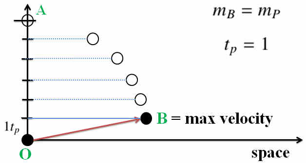
4.4. Each step along the time-line axis involves a \(1t_p\), in this example there are 6 steps and so 6 possible solutions along the space y-axis (and so 6 possible velocities), this also means that \(m_B\) can attain \(m_P\), but B (\(v = v_{max}\), \(m_B = m_P\), fig.4) can never attain the (horizontal axis) velocity \(c\) as always a minimum of 1 unit of Planck time is required. If we have a higher frequency, then we have more possible solutions bringing us closer to the horizontal axis and so traveling further in space. The higher the frequency of the particle, the higher the maximum potential velocity.

The vertical axis would be measured as \(1/\gamma\). For a particle that has only 6 divisions (6 steps from point to point), the maximum \(\gamma = 6\), with 12 divisions the maximum \(\gamma = 12\). To determine the maximum velocity that a particle can attain (y-axis = \(v/c\)) we simply calculate when that particle will have reached Planck mass, because from there it can go no faster. A small particle such as an electron has more divisions and so a higher \(\gamma\) and so can go faster in 3-D space than a larger particle such as a proton with a smaller \(\gamma\) (a smaller number of divisions). This is in contradiction to mainstream physics where the limiting factor is the energy required to reach a given \(\gamma\), whereas here the velocity limit occurs when the particle reaches Planck mass.

\(f_{electron} = m_P/m_e = 1836 \times f_{proton} = m_P/m_p\)

Hyper-sphere

We now replace the above with a 4-axis co-ordinate system, to illustrate this we use (\(h, x\)) axis with \(h\) as the time-line axis (of the expanding hypersphere) and \(x\) representing our 3-D space (\(x, y, z\)) with particles represented as semi-circles (cross-section). Note. I have been representing mass as relativistic mass, this is for convenience, in the hyper-sphere co-ordinate system there is only rest mass (particle frequency is constant and so the frequency of occurrence of the mass state is constant).

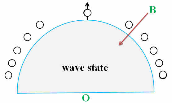
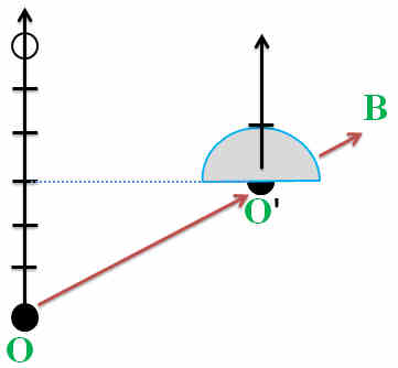
5.1. Depicted is particle B at some arbitrary universe time \(t\). B begins at origin O and its wave-state is pulled along by the hyper-sphere pilot wave expansion (fig.5, 6, 7).

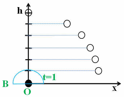
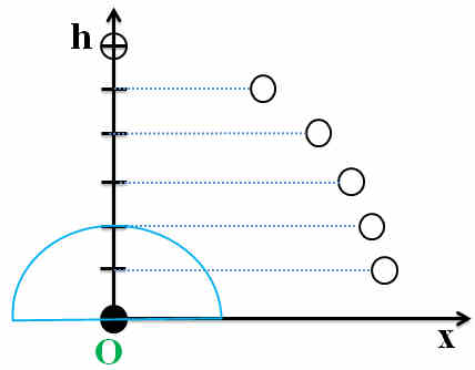
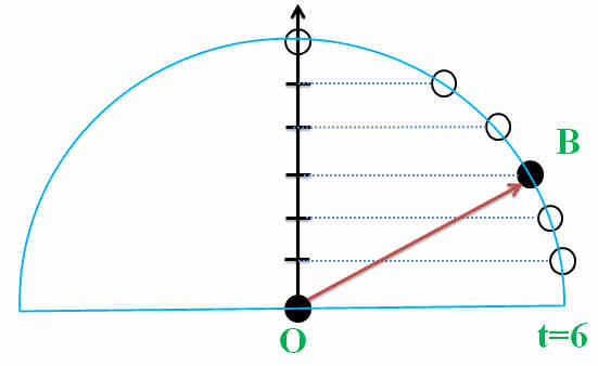
5.2. At \(t\) = 6, B collapses into the mass point state and has now defined co-ordinates within the hyper-sphere and these then become the new origin O' (fig.8), the above repeating ad infinitum \(t\) = 7, 8, … (fig.9, 10).

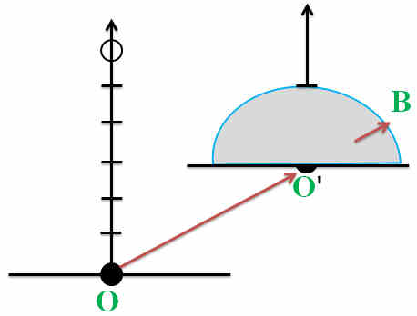
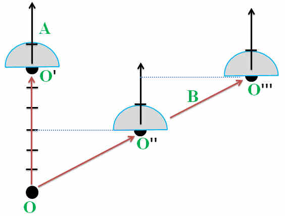
The process also repeats for A (fig.11). The universe hyper-sphere itself is then analogous to a particle presently in the wave-state whose origin O was the big bang (the universe however is still in the wave-state).

5.3. In the space-time diagram (fig.3) was depicted for A; (\(v = 0\), \(m_A = m_P/6\)) and for B; (\(v = 0.866c\), \(m_B = m_P/3\)). However in these graphs we find that as A and B have the same frequency, \(f = 6\), the lengths OA = OB = 6, this is because the hyper-sphere expands radially in 4-axis. As a consequence B can rightly claim that it is A whose velocity is at \(v = 0.866c\) and for B velocity \(v = 0\) (fig.12).

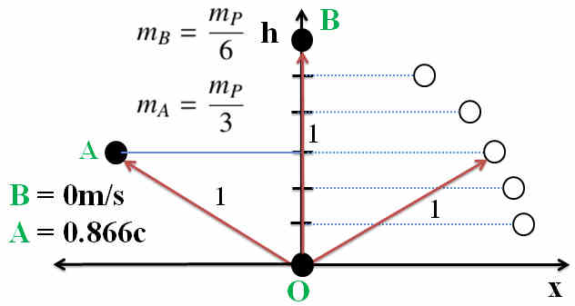
Both A and B are traveling at the speed of expansion (which translates to \(c\)) from the origin O. In the hyper-sphere coordinate system everything travels at, and only at, the speed of expansion as this is the origin of all motion, particles and planets do not have any inherent motion of their own, they are simply pulled along by this expansion.

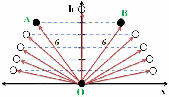
After 1 second both A and B will therefore have traveled the equivalent of 299792458 m in hyper-sphere co-ordinates from origin O (fig.13). Each of the 11 depicted solutions are equally valid as the radii are the same.

N-S axis, a particle internal rudder

Particles are assigned an internal N-S axis. In fig.14, as the universe expands, it stretches particle A (the position and motion of the wave-state are undefined). When time \(t = 6\), the wave-state collapses to the defined point-state, as determined by the N. This means that of all the possible solutions, it is the particle N-S axis which determines where the point-state will actually occur, with the hyper-sphere acting as a pilot-wave. We can imagine A as a small boat being pulled across a vast, expanding ocean. The N-S axis is the boat's rudder. It is the particle's internal orientation relative to the 4D expansion, and it dictates the particle's path along the 3D surface.

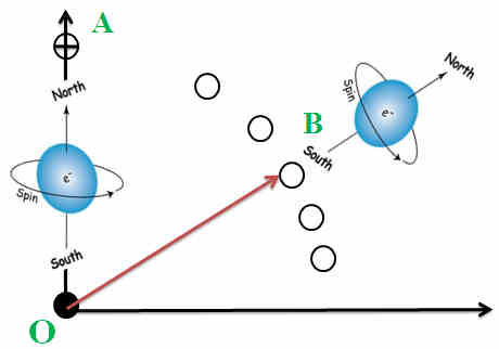
Thus if we can change the N-S axis orientation angle of B compared to A, then as the universe expands the B wave-state will be stretched as with A, but the point of collapse will now reflect the new N-S axis angle. B does not need to have an independent motion; B is simply being dragged by the universe in a different direction as the universe expands. Transferring physical momentum to B changes the N-S axis orientation. The radial universe expansion does the rest.

Photons and Cosmological Redshift

Information between particles is exchanged by photons. In this model, photons are unique: they do not have a mass point-state. and because they lack this mass state, they do not travel along the "timeline" h-axis in the same way as matter. Instead, they are "time-stamped" and travel laterally across the 3D surface of the expanding hypersphere. This behavior is the key to understanding what we observe. It explains how light moves and why we perceive cosmic redshift.

How Light Moves in the Hypersphere Model

The model describes our universe as the surface of an expanding 4-dimensional ball (the hypersphere). Conceptually on this expanding surface:

• Matter (like particles A and B) is carried "outward" with the expansion along the h-axis.
• Light (a photon) however travels "sideways" across this surface.

The photon's total speed through this 4D space—its "sideways" motion combined with the "outward" expansion—is always equal to the speed of light, \(c\).

When a photon travels for a long time across this expanding surface, its wavelength is stretched. This effect is what we observe as cosmological redshift.

Unlike a simple Doppler shift seen from an object moving through space, this cosmological redshift is a direct consequence of space itself expanding while the photon is in transit.

The geometry of the hypersphere model is powerful because it naturally reproduces the correct, observed formula for cosmological redshift. As the mathematical derivation in the Appendix shows, the "sideways" path of a photon on the expanding 4-sphere is mathematically identical to the standard cosmological formula:

(see Appendix. \(\lambda_{obs}/\lambda_{em} = R(t_{obs})/R(t_{em})\)).

Note: "The detailed mathematical derivation showing this equivalence involves concepts such as null geodesics and the FRW metric, and is provided in the Appendix."

Summary

Returning to our ABC particles, if photons (information) can only be exchanged along the horizontal axis (which represents the 3 axis of space; \(x, y, z\)), then ABC will only ‘see’ this horizontal information if ABC is relying on the electromagnetic spectrum. Instead of virtual co-ordinates OA, OB and OC and a constant time and velocity, the (\(x, y, z\)) axis will be able to measure only the horizontal AB, BC and AC (fig.15) as a 3-D space.

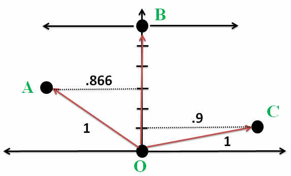
As for ABC there is no `depth' perception (the time-line h-axis), particle space will appear as a 3D space.

Furthermore time for ABC translates as motion, if there is no motion (no change of information states) in the (\(x, y, z\)) axis there will be no means to measure time, thus although the dimension of time for the 3-D space ABC world derives from the constant incremental expansion of the hyper-sphere, for observers it is actually a measure of change of state.

Appendix 1. Reconciling the Spiral and the Hypersphere

The model rests on two geometries: the 4-Axis Expanding Hypersphere (the physical container) and the Spiral of Theodorus (the algorithmic rule set) [3].

The hypersphere is the physical reality: it is the spatially finite container that expands linearly at the speed of light, \(c\), with every step of Planck time, \(t_P\).

The Spiral of Theodorus is the algorithm that tracks this expansion, with its components providing the formula for two distinct physical components of the universe:

1. Tracking the Scaffolding (Matter/Scale)
The linear length of the spiral, defined by the total number of elapsed Planck time units (\(t_{age}\)), tracks the physical scale of the universe and its dark matter content.

Scale Factor: The radius (\(R\)) of the expanding hypersphere (the scale factor, \(a(t)\)) is directly proportional to the total elapsed Planck time, \(t_{age}\) (\(R \propto t_{age}\)). This relationship defines the constant, linear expansion rate of the scaffolding itself, which remains consistent throughout all epochs.

Mass Density: The mass density of the non-baryonic Planck scaffolding (Dark Matter) is defined by the total mass (which scales with \(t_{age}\)) divided by the volume (which scales with \(t_{age}^3\)). Consequently, the mass density drops as \(1/t_{age}^2\).

2. Tracking the Observation (Radiation/CMB)
The radius and circumference of the spiral (\(\sqrt{t_{age}}\)) track the observable, energy-related properties.

CMB Temperature: As established in article 1, the Cosmic Microwave Background (CMB) temperature drops in inverse proportion to the spiral's radius (\(T \propto 1/\sqrt{t_{age}}\)).

Curvature and Force: The Casimir force, which in this model equates to the radiation energy density, is also defined by the spiral circumference (\(\propto \sqrt{t_{age}}\)).

This duality models the universe's evolution. The spiral radius \(\sqrt{t_{age}}\) dependence dominates the early radiation-dominated universe, leading to rapid changes in temperature and curvature. As the universe ages, the linear \(t_{age}\) growth continues, and the mass density's \(1/t_{age}^2\) drop becomes the dominant factor, defining the current matter-dominated universe. The spiral thus serves as the essential mathematical template that governs the transition between these two cosmological phases.

Appendix 2. Photon propagation as a null helix on the hypersphere

The photon is a key to this model and so this appendix has been included.

Photon absorption is not instantaneous: the absorber samples the incoming field over a finite interval of the cosmic expansion. In the hypersphere representation this process can be viewed geometrically as the motion of the photon along a null helix on the expanding 4-sphere that defines the Universe.

Let the radius of the hypersphere be \(R(t)\), with \(\dot R = c\). Points that are comoving in three-space move radially at \(c\) in the embedding frame but remain fixed in comoving coordinates on the 3-surface. A photon, by contrast, has both a radial and a tangential component of motion such that its total four-speed in the embedding space remains exactly \(c\). The trajectory satisfies the null condition

where \(d\chi\) is the infinitesimal angular displacement on the 3-surface. Hence

Integrating gives the photon path

which is equivalent to the usual FRW null geodesic condition \(c\,dt/a(t) = d\chi\) with \(a(t) \equiv R(t)\).

In the embedding space the photon's worldline thus traces a helix: the radial component \(\dot R = c\) represents the cosmic expansion, while the tangential component \(R(t)\dot\chi\) represents the propagation of the photon across the 3-surface. The combined motion satisfies

so the path is null in the four-dimensional metric. Earlier segments of the helix correspond to smaller radii \(R(t_{\mathrm{em}})\)—the geometric past—while the intersection of the same worldline with the present hypersphere radius \(R(t_{\mathrm{obs}})\) corresponds to the photon observed "now." The photon is therefore never left behind: it always resides on the expanding surface, though its tangential projection redshifts according to

identical in form to the standard cosmological redshift relation.

From this perspective the Doppler effect can be interpreted as a local tangent-space picture of the same process: the finite absorption time corresponds to a short arc of the null helix, during which the absorber moves radially outward with the expanding surface while the photon advances tangentially across it. The observed redshift thus reflects the geometry of the helix rather than a literal "stretching" of the photon through space.

Connection to the standard FRW metric

The hypersphere construction can be written in the familiar FRW form by identifying the hypersphere radius \(R(t)\) with the cosmological scale factor \(a(t)\). Embedding the three-dimensional spatial surface of the Universe in a four-dimensional Euclidean space with coordinates \((w,x,y,z)\), the induced line element on the 3-surface satisfies

so that

Differentiating and restricting to the surface yields

which is the Robertson-Walker metric for a closed (\(k=+1\)) universe when written as

Here \(a(t) \equiv R(t)\) and the coordinate transformation \(r = \sin\chi\) maps the hypersphere coordinates to the usual FRW form. For small curvature, \(\chi \ll 1\) and \(r \simeq \chi\), so the spatial metric becomes locally Euclidean:

the standard flat-FRW metric. The null condition \(d\Sigma^2 = 0\) gives the same photon trajectory equation as before,

integrating between emission and observation times yields the conventional redshift law,

Thus, the hypersphere model and the standard FRW formulation are mathematically equivalent in the continuum limit: the radial expansion of the hypersphere corresponds to the increase of the FRW scale factor, and the tangential motion of photons on the hypersphere surface reproduces the same null geodesics and redshift relations. At small curvature or over local regions of the Universe the metric reduces smoothly to Minkowski space, ensuring consistency with special relativity.

From Planck ticks to the continuum

The model is fundamentally defined as an evolution in integer Planck steps (ticks), \(t_n = n t_P\), with geometric and physical variables specified as discrete sequences \(X_n\). In the text we frequently write continuum expressions (derivatives and integrals). This Appendix shows why those continuum formulae are an excellent effective approximation.

Define the forward difference

A discrete evolution law may be cast as

with \(F_n\) the update per tick. Introduce the interpolating function \(X(t)\) with \(X(t_n)=X_n\) and apply Taylor's theorem:

for some \(\xi \in (t, t+t_P)\). Rearranging yields

so the finite difference equals the continuum time derivative plus an error term of order \(t_P |\ddot X|\). If \(X\) varies on a characteristic timescale \(T\) then \(\ddot X \sim X/T^2\) and the relative error in the derivative is of order \(t_P/T\). Thus the continuum approximation is justified whenever \(t_P \ll T\). For cosmological quantities \(T\) is enormous when compared with \(t_P\): taking the Planck time \(t_P \approx 5.39 \times 10^{-44}\,\text{s}\) and the present age \(T \sim t_{\text{now}} \approx 4.6 \times 10^{17}\,\text{s}\) gives \(t_P/T \sim 10^{-60}\). Consequently the Taylor remainder is utterly negligible and ordinary calculus provides an accurate description.

Two further points follow:

• Averaging and absorption. Observables such as absorbed photon frequency are measured over an interaction (coherence) time \(\tau_{\text{abs}}\) that typically spans many Planck ticks. The measured quantity is the time average \[ \overline{f} = \frac{1}{\tau_{\text{abs}}} \sum_{n=n_0}^{n_0+N-1} f_n t_P \approx \frac{1}{\tau_{\text{abs}}} \int_{t_0}^{t_0+\tau_{\text{abs}}} f(t)\,dt, \] with \(N = \tau_{\text{abs}}/t_P \gg 1\), so discrete sampling converges to the continuum integral.
• Stochastic fluctuations. If microscopic updates include small random components with variance \(\sigma^2\) per tick, then by the central limit theorem the accumulated fluctuation after \(N\) ticks scales as \(\sigma\sqrt{N}\), while the mean scales as \(N\). Hence the fractional fluctuations scale as \(1/\sqrt{N}\). With \(N \sim 10^{60}\) these are \(\lesssim 10^{-30}\) and cosmologically irrelevant.

In summary: the continuum calculus used in the main text is the justified coarse-grained, effective description of an underlying Planck-tick discrete model, provided one examines physics on timescales \(T \gg t_P\) (the regime relevant for all cosmological observables in this work). Where necessary, difference equations can be written down explicitly and the small correction terms (of order \(t_P/T\)) retained to bound departures from the continuum limit.