Part 1b: The Minimal Complexity Algorithm of the Planck Scaffolding

1. Introduction: The Simulation Paradigm

The correlation between the Planck unit scaffolding and the Cosmic Microwave Background established in Article 1a [1] suggests that the universe may operate as a discrete computational process. In standard physics, spacetime and quantum fields are fundamental. In the simulation framework the discrete computational step is fundamental, and continuous or quantum-mechanical features are emergent properties of sufficiently many discrete accumulations.

To formalise this we require a minimal complexity algorithm. The universe cannot be pre-initialised with a "bag of constants"; primary units and constants must be generated on demand by the algorithm's own state machine. This supplement details the internal mechanics of a single step, showing that the primary physical units are structurally forced by the geometry of discrete counting. Familiarity with the main article [1] is assumed.

On the status of this text. The architecture described here is also implemented as a running program, and where the two disagree the program is the reference. Prose can be read two ways; code cannot. Function names are cited in the text as like_this(), referring to spiral_branch.py, there are also 2 accompanying animation programs; tau_animation.py and branch_animation.py.

1.1 Axioms of the Minimal Complexity Algorithm

The derivations in this paper rest on two tiers of assumption, kept separate because they carry different epistemic weight.

Counters. Two counters suffice:

\(t\) is the number of 'physical' steps (each step deposits a set of Planck units). \(B = 15\).

Tier 1: Foundational axioms. These define the minimal computational framework. No empirical constant appears in Tier 1; the only numbers are structural integers and the mathematical consequences of the postulated geometry.

Structural identification. Because the deposit is exactly one unit and \(t\) never resets, the running sum telescopes exactly, with no asymptotic correction at any \(t\):

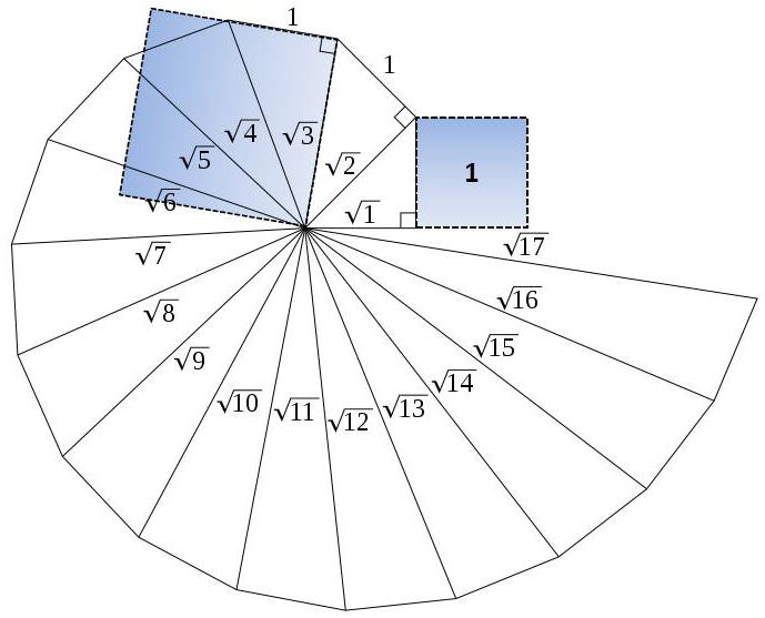
Geometrically this is the primal box: the square erected on the spiral radius has side \(\sqrt{t}\) and area \(t\), so each completed step adds exactly one unit box. The side is the wave-state quantity (a square root, sign- and phase-carrying); the area is the point-state quantity (a positive integer). This axiom fixes only the modulus \(|z_t|\); the phase of \(z_t\) is set independently by Axiom 3. In particular a complex radius is permitted --- \(r_t^{2}=t\) would force the phase into \(\{0,\pi\}\), but the derived condition is \(|z_t|^{2}=t\), which admits any phase.

Remark (open loops deposit nothing, and branches deposit nothing). The deposit is conditioned on loop completion. A \(\tau\)-loop that remains open accumulates phase and contributes no box until it closes: a never-closing loop (photon) deposits nothing at any \(t\). A branch is a single \(\tau\)-loop running \(\psi\) times slower than the scaffolding loop (Section 5); it has therefore not completed its first \(\Omega^{B}\) and generates no new Planck units at all. At closure it marks an existing box rather than depositing a new one, so this axiom's one-unit rule is not violated by branch closure --- branch closure is not a scaffolding collapse.

Structural identification. With \(|z_t|=\sqrt{t}\) this fixes the phase increment as \(\Delta\Theta_t \to 1/\sqrt{t}\), and together with Axiom 2 it forces the Theodorus step operator \(S_t = 1 + i/\sqrt{t}\) (Section 3.1) --- a derived structural consequence, not a further postulate. Note that the conserved quantity is \(r\omega \to 1\), a constant tangential speed; it is not angular momentum, for which \(r^{2}\omega\) would have to be constant and in fact diverges.

Structural identification. The equation is the defining generator of the exponential; its solution is \(\tau(s)=e^{s}\), so \(\tau(1)=e\). Thus \(e\) is not derived from more primitive axioms --- it is the natural coordinate of the logarithmic action \(\Delta(\ln\tau)=1\) imposed by the calibration. The reset is a selected convention, not a theorem: the bare differential equation is equally consistent with a \(\tau\) that accumulates. It is however the reading under which Axiom 8's closure condition holds at every cycle rather than only the first.

Structural identification (eigenvalue). The solution vanishing at \(u=0\) is \(w=A\sin(\sqrt{\lambda}\,u)\); imposing \(w(1)=0\) forces \(\sqrt{\lambda}=k\pi\). The lowest mode is

The eigenvalue is \(\lambda_{1}=\pi^{2}\); \(\pi=\sqrt{\lambda_{1}}\) is the derived wavenumber. This distinction matters downstream: the render invariant's \(\pi^{2}\) is \(\lambda_{1}\) carried through intact, not a secondary quantity squared.

Structural identification (the half-cycle). The phase accumulated over one complete loop is

One \(\tau\)-loop is a half cycle. Consequently the complex wave-state acquires a factor \(e^{i\pi}=-1\) per loop, and the collapse state is \(-\Omega^{2}\) rather than \(+\Omega^{2}\) (Section 3.4). Two loops are required to return to \(+\Omega^2\). This is the origin of the phase convention used throughout, of the collapse sign, and --- via the \(4\pi\) periodicity it induces --- of spin-\(\tfrac12\) in Section 5.

Structural identification (synchronisation). Because \(t\) advances only in whole units and there is no clock external to the lattice, any process that closes onto the spiral must close on a spiral step. This is a genuine constraint, not a convenience: it requires the closure count of any branch to be an exact integer number of steps (Section 5), and it is what makes \(t\) a single global index --- "now" is one value for the whole lattice, which is the sense in which the scaffolding is uniform everywhere. Note, although we have a formula for the electron \(\psi_e\)

the value for the fine structure constant alpha is not known with enough precision to determine the exact value of \(\psi_e\) and so this integer conjecture cannot be tested.

Tier 2: Structural postulates. Axioms 1--6 establish the discrete recursion, the domain duality, the tick hierarchy, and the identification of \(e\) and \(\pi\) as the natural coordinates of the \(\tau\)-loop. They do not fix a unique way to combine \(\pi\) and \(e\) into a single expansion eigenvalue

The following closes that gap. Both the functional form and the point at which it is evaluated are postulated, not derived.

Structural identification (gain versus endpoint). \(A(1)=\Omega^{1}\) and \(A(e)=\Omega^{2}\), so the gain per cycle is \(\Omega\), while \(\Omega^{2}\) is the endpoint value. Over the \(B\) cycles of one spiral step the accumulated gain is therefore

not \(\Omega^{2B}\). Combined with the half-cycle phase, the full complex state at collapse is \(\Psi(e)=\Omega^{2}e^{i\pi}=-\Omega^{2}\). At closure the state runs from \(-\Omega^{2}\) to \(+\Omega^{2}\); two cycles to return. The amplitude resets with \(\tau\) at each cycle boundary, so this is a return of the whole state, not merely of its sign.

Remark (on computing \(e\) and \(\pi\)). These are computable from the model's own primitives by series summation, requiring no external lookup, unlike \(\alpha\). A Basel summation (\(\sum k^{-2}\to\pi^{2}/6\)) for example may evolve with the spiral steps \(t\) providing the integers:

2. The Minimal Complexity Algorithm

We model the universe as a state machine driven by a WHILE loop. The physical clock advances only when the internal evaluation (the \(\tau\)-loop) completes and the state collapses. The architecture consists of two coupled fibers:

• Phase-amplitude fiber (Axioms 1, 4, 5): a continuous logarithmic spiral in the complex plane, governed by \(e\) and \(\pi\), whose amplitude matures to \(\Omega^{2}\) while its phase advances by \(\pi\) --- a half cycle, so the state collapses to \(-\Omega^{2}\).
• Coordinate fiber (Axioms 2, 3): a discrete algebraic spiral (Theodorus), governed by orthogonal right-triangle accumulation, depositing one unit per spiral step \(t\).

These fibers are not derivable from one another; they are orthogonal aspects of the same collapse event, coupled through the counters and the render invariant \(\pi^{2}\Omega^{15}\).

2.1 Domain partition

The following distinction organises the remainder of the paper and determines which methods transfer between sections:

A corollary worth stating, because it prevents a recurring confusion: a spiral-domain description of a branch object is a projection, not a definition. Descriptions of the wave-state phrased in point-state vocabulary --- "no fixed coordinates", "a probability density" --- are what the spiral domain is obliged to say about something it cannot represent, not statements about the object itself. The resemblance to the standard quantum-mechanical account is therefore expected rather than coincidental.

2.2 The simulation loop

t = 0;                  // spiral step; NEVER resets. t IS the Planck step.
n = 0;                  // internal tau-cycle counter; resets at B.
B = 15;                 // minimal integer base (Section 4.2)

// The Omega equation is hardcoded into the simulation source-code
hardcoded_Omega_equation = sqrt(pi^e * e^(1-e));

WHILE (simulation_active) {

    // 1. RUN ONE TAU-CYCLE
    // pi and e are computed from the model's own primitives by series
    // summation. WHICH series is an open structural choice.
    pi_n = update_series_pi(t);
    e_n  = update_series_e(t);
    Omega_n = sqrt( (pi_n)^(e_n) * e_n^(1 - e_n) );

    // tau RESETS to 1 at the start of every cycle (Axiom 4)
    tau = 1;
    WHILE (tau < e) {
        // amplitude  A = Omega^(ln tau + 1):  Omega  ->  Omega^2
        // phase      phi = pi ln tau       :  0      ->  pi   (HALF cycle)
        expand_spiral(Omega_n, tau);
        rotate_spiral(Omega_n, tau);
        tau = tau + delta_tau;
    }

    // 2. CYCLE BOUNDARY
    // amplitude has matured to Omega^2 and the phase factor is e^{i pi},
    // so the collapse state is -Omega^2. The GAIN this cycle is Omega,
    // not Omega^2; B cycles therefore accumulate Omega^B = Omega^15.
    collapse_wave_state();
    n = n + 1;

    // 3. RENDER EVENT: when the internal counter completes B cycles
    if (n == B) {
        n = 0;                  // internal counter resets
        t = t + 1;              // spiral step advances
        deposit_primal_box();   // |z_t|^2 = t exactly
        render_physical_units();  // unpack pi^2 Omega^15 into P, M, T

        // 4. DERIVED QUANTITIES computed on demand from M, T, P and alpha.
        //    Internal scale is fixed by the dimensionless anchor f(y).
        compute_derived_quantities();
    }
}

3. The Primary Units: From Structural Postulates to the Render Event

In Article 1a, the mass/length domain scales linearly with the step index \(t\), while the radiation domain scales as \(\sqrt{t}\). This domain duality is not imposed on the algorithm; it is a mathematical consequence of the Theodorus step operator.

3.1 Derivation of the Theodorus Step Operator

The geometry of the Spiral of Theodorus is not an arbitrary starting assumption but a consequence of Axioms 2 and 3. Its content is independent of the \(\tau\)-loop (Axioms 4--5); their coupling in time, rather than content, is made precise in Section 3.8.

By Axiom 2, each step adds exactly one unit of real coordinate and an orthogonal imaginary phase: if the squared coordinate amplitude is \(t\), the real increment advances it to \(t+1\). By Axiom 3, the phase rate is the reciprocal of the coordinate amplitude in the mature limit; as the amplitude is \(\sqrt{t}\), the phase increment must be \(1/\sqrt{t}\). For small angles the tangent of the increment equals the ratio of imaginary to real components, and since the real component is \(1\), the unique operator satisfying both conditions is

The recursion \(z_{t+1}=z_tS_t\) (with \(z_1=1\)) is therefore a derived theorem, not an independent postulate. Its modulus is

so by induction the squared amplitude telescopes exactly to \(|z_t|^{2}=t\). The real component advances \(|z_t|^{2}\) by exactly one integer per step, and \(M=1\) is the read-out of that real projection.

3.2 The Phase Increment and Domain Duality

The argument of \(S_t\) is \(\arctan(1/\sqrt{t})\), so the accumulated phase after \(t\) steps is

the asymptotic form following from Euler--Maclaurin summation, with \(K\) the Theodorus constant. The phase grows as \(\sqrt{t}\), not as \(t\): it belongs to a different scaling class from the squared amplitude. Separating the operator,

the real part defines coordinates (\(|z_t|^{2}=t\), integer), governing mass, volume and macroscopic time; the imaginary part generates phase (\(\Theta_t\approx2\sqrt{t}\), irrational), governing wavelength, frequency and temperature [1]. At this level the imaginary component has no spatial coordinate to correlate with: an independent spatial manifold does not yet exist.

3.3 Symmetry Conservation and the Render Event

The \(\tau\)-loop (logarithmic, transcendental) and the Theodorus spiral (algebraic, discrete) are geometrically incompatible as descriptions of a single curve. They are orthogonal fibers of the simulation state, coupled at the render event.

During the sub-Planckian sequence (\(n=1\) to \(B-1\)) the \(\tau\)-loop accumulates a dimensionless invariant

conserved in the sense that it may be repackaged without altering its value. The quantities \(P,M,T\) are not independently derived here; they satisfy the invariant subject to two constraints: the phase-balance equation \(P^{15}T^{2}/M^{12}=I\), and integrality of the unit-number exponents \(\theta(\cdot)\).

The parameterisation (imported from Article 6 [5])

carries the assignment of \(\Omega\) and \(\pi\) content to \(P\), \(M\) and \(T\). Of the quantities here, only scalars \(r\) and \(v\) constitute a genuine gauge choice --- bookkeeping variables rescalable without altering any prediction --- unlike the \(\Omega,\pi\) assignment, which is fixed. The render event is therefore a threshold crossing rather than a symmetry-breaking process: \(I\), well-defined throughout the sub-Planckian phase, is unpacked into physical containers once the integer lock is first satisfied.

3.3.1 The invariant is a group volume

The invariant admits an exact geometric reading. Since \(\Omega^{15}=(\Omega^{5})^{3}\), and \(\mathrm{Vol}(\mathbb{RP}^{3})\) at radius \(a\) is \(\pi^{2}a^{3}\),

while the double cover has exactly twice that volume,

Both translation scalars cancel identically in the phase-balance equation that fixes \(I\): substituting the scalar expressions, the exponents of \(r\) in \(P^{15}T^{2}/M^{12}\) sum to \(30+18-48=0\) and those of \(v\) to \(-12+12=0\). The cube is therefore a spatial dimension count, not an unexplained power. The render lands on the volume of the rotation group; the full state space is its double cover. \(\Omega^{5}\) is identified as the monopole quantum (Section 5), so the radius is not an arbitrary length. And the factor \(2\) between \(SO(3)\) and \(SU(2)\) is the same factor that appears as the \(\tau\)-loop's half cycle, as the distinction between the observable (\(2\pi\)-periodic) and the configuration (\(4\pi\)-periodic), and as mass seeing \psi while spin sees \(2\psi\).

3.3.2 The \(\Omega\) grading: \(\Omega^{2}\times\Omega^{3}=\Omega^{5}\)

The powers of \(\Omega\) carried by the physical quantities partition the table into the two domains and their product. Reading the \(\Omega\) content directly from Table 1:

Since \(K=AV/2\pi\) by definition,

so the grading is realised by the statement that temperature is current times velocity. The \(\Omega^{3}\) in \(A\) is likewise forced: \(V^{3}\sim(\Omega^{2})^{3}=\Omega^{6}\) and \(P^{3}\sim\Omega^{3}\), so \(A\sim V^{3}/P^{3}\sim\Omega^{3}\).

Where \(\Omega^{2}\) comes from. It is the closure amplitude of the \(\tau\)-loop itself: \(A(\tau)=\Omega^{\ln\tau+1}\) matures to \(\Omega^{2}\) at \(\tau=e\) (Axiom 8). The mass-domain grade is therefore the amplitude at which the loop collapses.

Consequences. \(\Omega^{5}\) is the monopole quantum --- the product of one mass-domain and one charge-domain factor --- which is why \(\sigma_e\) and \(\sigma_t\) both carry \(\Omega^{5}\) (Section 5). And \(\Omega^{15} = (\Omega^{5})^{3}\) is three such quanta, which is why the render invariant \(I=\pi^{2}\Omega^{15}\) is a volume of a three-dimensional space.

3.3.3 The unit number is fixed by the scalars

Writing each quantity's scalar content as \(r^{a}v^{b}\),

with \(r,v\) carrying unit numbers \(8\) and \(17\). For example; \(r^4 v^{-1} \implies 4\times 8 - 17 = 15\); \(r^{17} v^{-8} \implies 17\times 8 - 8\times 17 = 0\).

Consistency is internal: \(\theta(V)=17\) because \(V\)'s scalar is \(v\), and \(\theta(P)=16=2\times8\) because \(P\)'s scalar is \(r^{2}\). The unit-number check and the scalar check are the same check.

3.4 The render invariant \(\pi^{2}\Omega^{15}\), and the sign it carries

3.4.1 \(\pi^{2}\) is an eigenvalue, not a squared wavenumber

Under Axiom 5 the internal oscillation along the logarithmic coordinate \(u = \ln\tau \in [0,1]\) satisfies

whose eigenvalues are \(\lambda_m = m^{2}\pi^{2}\). The fundamental is \(\lambda_1 = \pi^{2}\), with \(\pi = \sqrt{\lambda_1}\) as the derived wavenumber. The \(\pi^{2}\) in \(I = \pi^{2}\Omega^{15}\) is the eigenvalue itself, carried through intact.

3.4.2 The deposit alternates in sign

Each \(\tau\)-loop advances the phase by \(\varphi = \pi\ln e = \pi\), so its closure carries the factor \(e^{i\pi} = -1\) and the wave-state collapses to \(\Psi(e) = \Omega^{2}e^{i\pi} = -\Omega^{2}\) (Axiom 8). A single Planck step comprises \(B = 15\) such loops, so after \(t\) Planck steps the accumulated factor is

The deposit therefore alternates:

The sign is fixed by the step parity, and half of all deposits are negative. The lattice deposits one unit of \(I\) per step, additively, giving \(tI\) after \(t\) steps. Every deposit is the same size; only its orientation flips.

3.4.3 Two returns, at two scales

Only the second is resolvable, since a single \(\tau\)-loop is not an event the lattice records. The observable spinor period is therefore two Planck steps, and it exists only because \(B\) is odd.

3.4.4 Where the two-step state is held

A state with a two-step period requires a configuration space in which a \(4\pi\) rotation closes but a \(2\pi\) rotation does not. That space is the 3-sphere: \(S^{3} \cong SU(2)\) double-covers \(SO(3)\), and its volume is exactly twice that of \(SO(3)\): \(\mathrm{Vol}(S^{3}) = 2I = 682\,304.6874\). The alternating sign is the position of the state on \(S^{3}\): a continuous trajectory that has covered \(SO(3)\) once after one Planck step and twice after two, returning to its starting point only on the second pass.

3.5 Emergence of \(e\), \(\pi\), and \(\Omega\)

3.5.1 Identification of \(e\): the loop boundary

One unit of logarithmic action is required within the \(\tau\)-loop. Since \(A(\tau)=\Omega^{\ln\tau+1}\), the change in \(\Omega\)-exponent is \(\Delta k=\ln\tau_{\text{final}}=1\), whose unique solution is \(\tau_{\text{final}}=e\). Euler's number is the natural coordinate of the logarithmic action imposed by Axiom 4.

3.5.2 Identification of \(\pi\): the boundary phase

The phase-generating oscillation is a standing wave in \(u=\ln\tau\), \(w(\tau) = \sin(\pi\ln\tau)\), vanishing at both endpoints of \(u\in[0,1]\). The phase accumulated over the full loop is

and the Planck time unit \(T=\pi\) counts this half cycle: one loop advances the phase by \(\pi\), not \(2\pi\), so the complex state acquires a factor \(e^{i\pi}=-1\) and collapses to \(-\Omega^{2}\). Two loops are required to return.

3.5.3 Definition of \(\Omega\) via the capacity functional

Following Axiom 7,

evaluating at the loop boundary \(x=e\):

taking the positive root. The \(\tau\)-loop evaluates \(A(\tau)=\Omega^{\ln\tau+1}\), spanning \(\Delta\ln\tau=1\) and terminating at \(\tau=e\), where \(A(e)=\Omega^{2}\). The gain per cycle is \(\Omega\), so \(B\) cycles accumulate \(\Omega^{B}=\Omega^{15}\).

3.6 The Momentum Invariant in the Continuum Limit

In the continuum limit the amplitude is \(\sqrt{t}\) and the phase \(2\sqrt{t}\), so

This product locks to unity for all \(t\): Planck momentum is an emergent, scale-invariant property of the mature lattice. Note that the conserved quantity is \(r\omega\to1\), a constant tangential speed, and not angular momentum.

3.7 The Quantization of Action

Define the step action \(a_{t}\) as the product of coordinate amplitude and phase increment:

The action per step approaches exactly \(1\) as the lattice matures: the quantum of action \(\hbar\) is an asymptotic property of the expanding spiral, not a primordial axiom.

3.8 Clock and Counter: The Disk Construction

The relationship between the \(\tau\)-loop and the spiral is asymmetric: Axiom 8 is explicit that the \(\tau\)-loop's boundary condition advances the counter. The Theodorus recursion has no completion condition of its own; it describes what is deposited at a step, not when one occurs. The \(\tau\)-loop is the pacemaker and the spiral is read out at each closure.

Consider the two components directly:

Lemma 1 (Polar reformulation). \(z_t = r_t e^{i\Theta_t}\) for all \(t\ge1\), where \(z_t\) is generated by \(z_{t+1}=z_tS_t\), \(z_1=1\).

Proof. By induction. Base: \(r_1=1\), \(\Theta_1=0\), so \(z_1=1\). Step: assume \(z_t=r_te^{i\Theta_t}\). Then \(|z_{t+1}|=r_t\sqrt{1+1/t}=\sqrt{t+1}=r_{t+1}\) and \(\arg(z_{t+1})=\Theta_t+\arctan(1/\sqrt{t})=\Theta_{t+1}\). \(\blacksquare\)

Pitch. Since \(\Theta_t\to2r_t\), one full turn (\(\Delta\Theta=2\pi\)) corresponds to a radial advance \(\Delta r = \pi\). The spiral is asymptotically Archimedean with pitch exactly \(\pi\): successive turns lie \(\pi\) Planck lengths apart.

4. Physical Constants from \(\Omega\) and \(\alpha\)

4.1 The Base-15 Phase Closure

While one \(\tau\)-cycle generates an \(\Omega\) gain, constructing the primary physical units requires simultaneous alignment of multiple dimensional phases. A minimum of \(B=15\) cycles is required, so the master scalar for one complete structure is \(\pi^{2}\Omega^{15}\):

Substituting the scalar parameterisations, \(r\) and \(v\) cancel completely, showing independence of internal gauge choices.

4.2 Diophantine System with Constraints

Initial conditions:

Substituting \(\theta_T=-2\theta_M\):

Since \(\gcd(15,16)=1\), every integer solution is:

Pairwise distinctness holds automatically for every non-zero \(k\). As \(\theta_P = {\theta_r}^2\), then \(\theta_r = 8, \theta_v = 17\).

4.2.1 The general solution and \(k\)-scaling

The condition admits the family \(\theta_M=15k\), \(k\in\mathbb{Z}^{+}\), each \(k\) corresponding to \(k\) complete copies of the fundamental structure. While higher-\(k\) modes are valid overtones, \(k=1\) is the unique minimal mode and is taken as the physical base. The positive sign is forced by the monotonicity of coordinate accumulation (\(M\) grades accumulating quantity).

5. Branch Physics

5.1 Scope and status

Section 4 describes the Planck scaffolding: the \(\tau\)-loop, the base-\(B\) integer lock, and the spiral of primal boxes. That scaffolding is \(\alpha\)-free. Every quantity entering it (\(M, T, P, V, L\)) is constructible without the fine-structure constant; only \(A\) and \(K\) carry \(\alpha\). This section concerns what happens off the scaffolding, in the domain where \(\alpha\) does appear: the branch, or baryonic, domain.

5.2 Two autonomous closure engines

The central structural claim of this section is that the branch is not a new mechanism. It is the same mechanism as the \(\tau\)-loop, running with a different closure target.

The scaffolding \(\tau\)-loop rotates and expands under a fixed rule set until it reaches its closure value \(I = \pi^{2}\Omega^{15} = 341152.343709\ldots\), whereupon it collapses and resets. The branch runs the same way, but closes at \(\psi = \frac{\sigma_{e}^{3}}{2T}\), where \(\sigma_{e}\) is the monopole amplitude. Neither engine counts: each accumulates under its rule until a geometric condition is met.

5.3 The monopole quantum \(\Omega^{5}\)

The mass domain carries \(\Omega^{2}\) and the charge domain \(\Omega^{3}\); their tensor product is the dual-domain node

This is the smallest object with simultaneous presence in both domains ($Q^5$ monopole). Since \(\Omega^{15}=\bigl(\Omega^{5}\bigr)^{3}\), the \(\Omega\)-content of the render invariant is exactly three monopole quanta.

The monopole amplitude. From the MLTA objects, with \(A\) the current (\(\theta=3\)) and \(L\) the length (\(\theta=-13\)),

The normalised monopole amplitude is

\(\alpha\) enters \(\sigma_{e}\) exactly once, distinguishing branch from scaffolding.

5.4 Why \(\psi\) is a cube

Three separate lines converge on the same cube:

1. Composition. The electron is the triplet \(DDD=(AL)^{3}/T\) with \(D=\sigma_{e}\): three monopoles.
2. Coincidence count. If three monopole phases have per-tick coincidence probability \(p\approx 1/\sigma_{e}\), the expected waiting time to a simultaneous coincidence is \(\mathbb{E}[W_{3}]\approx\sigma_{e}^{3}=1.501396\times10^{23}\).
3. Unit-number closure. Only the combination \((AL)^{3}/T\) has vanishing unit number and unit scalars: \(\theta\bigl[(AL)^{3}/T\bigr]=3(-10)-(-30)=0\), and \(\left(\frac{r^{3}}{v^{2}}\right)^{3}\frac{v^{6}}{r^{9}}=1\).

Dividing by the time unit \(2T=2\pi\) gives the invariant:

Alternative route. With \(\sigma_{t}=3\alpha^{-2}AV/(2\pi^{2})=2^{6}3\pi^{2}\alpha^{-1}\Omega^{5}\) (\(\theta=+20\)), the alternative composition \(DUU\) gives \(\psi=(2T)\,\sigma_{t}^{2}\,\sigma_{e} = 2^{20}3^{3}\pi^{8}\alpha^{-3}\Omega^{15}\), identical to the above. Electron and positron share one geometry.

5.5 The holonomy constraint and the degrees of freedom

The three monopole phases \(\phi_{1},\phi_{2},\phi_{3}\) satisfy

5.5.1 The phase convention is fixed by the model

With \(\phi_{j}(k)=\pi n_{j}k/\psi\) (\(n_{j}\in\mathbb{Z}\)), the holonomy at closure reads

5.5.2 Precession, read off the dynamics

The N--S azimuth is \(\Delta=\phi_{3}-\tfrac12(\phi_{1}+\phi_{2})\), giving precession per cycle:

5.5.3 The degree-of-freedom count

The ansatz \(z_{1}=\sqrt{\tfrac23}\,e^{i(\phi_{1}+\phi_{2})/2}\), \(z_{2}=\sqrt{\tfrac13}\,e^{i\phi_{3}}\) fixes \(n_{z}=|z_{1}|^{2}-|z_{2}|^{2}=\tfrac13\), \(\theta=\arccos\tfrac13=70.5288^{\circ}\). The reachable states form a latitude circle on the Bloch sphere.

5.5.4 Where spin-\(\tfrac12\) actually comes from

The 3D domain is the surface of the expanding hypersphere \(S^{3}\cong SU(2)\), which double-covers \(SO(3)\). A \(2\pi\) rotation in \(SO(3)\) lifts to a path in \(S^{3}\) that closes only after \(4\pi\). Spin-\(\tfrac12\) is an intrinsic topological property of the space itself.

5.6 The branch cycle

Definition 1 (Branch cycle). Let \(k\) index ticks within one branch cycle:

• Point-state, \(k=0\), duration \(1\,t_{P}\). The branch coincides with the spiral. \(\theta=0\); one Planck-mass unit is present.
• Wave-state, \(k=1,\dots,\psi\), duration \(\psi\,t_{P}\). The branch is off the spiral. There is no mass density and no position. The three monopole phases evolve under \(A(\tau)=\Omega^{\ln\tau+1}\).
• Closure, at \(k=\psi\): holonomy is satisfied, wave-state collapses, and cycle restarts.

Mass as a duty cycle. Time-averaged mass is

The mass ratio is a duty cycle of point-state manifestation.

5.7 Marking versus deposition

5.8 Autonomy of the branch clock

Electron mass is constant over cosmological time. Since \(m_{e}=m_{P}/\psi\), \(\psi\) is independent of spiral index \(t\). Total phase rate is

5.9 Photon, positron, annihilation

• Photon. A branch whose \(\tau\)-loop never closes. No point-state occurs, duty fraction is \(0\), propagates at \(c=\ell_{P}/t_{P}\).
• Positron. The \(DUU\) composition (\(\theta=+30\)), sharing identical \(\psi\) with \(DDD\). Differing in charge structure only.
• Annihilation. Destructuring of the closure condition so neither branch reaches a point-state, converting both into non-closing loops (photons).
• Marked versus unmarked boxes. The electron is a branch-state phenomenon; the spiral provides the Planck unit scaffolding.

6. Conclusion

The CMB correlations of Article 1a are presented here as the macro-scale asymptotic results of a constrained minimal-complexity algorithm operating at the Planck scale. By modelling the universe as a continuous \(\tau\)-function evaluating a hardcoded \(\Omega\) equation, pre-initialised constants and externally imposed clocks are eliminated. The discrete step and mass unit \(M=1\) are forced by geometry; \(T=\pi\) follows from Axiom 5; and \(\Omega\) is fixed by Axiom 7. With two empirical inputs (\(\alpha\) and \(f(y)\)), the framework provides a rigorous candidate mathematical foundation for the Simulation Hypothesis.

Appendix A: The Hypersphere

A.1 The 3D surface is \(S^{3}\), and this is load-bearing

The observable 3D universe is the surface of the expanding hypersphere \(S^{3}\cong SU(2)\). \(SO(3)=S^{3}/\{\pm1\}=\mathbb{RP}^{3}\). A \(2\pi\) rotation in 3D space lifts to an open path on \(S^{3}\), closing after \(4\pi\).

A.2 Expansion without a dark-energy term

Taking \(R\propto\sqrt{t}\) and elapsed time \(\propto\sqrt{t}\), scale factor \(a\propto\text{time}\), yielding \(H = \frac{\dot a}{a} = \frac{1}{\text{time}}\) without dark energy [3].

A.3 The holographic reading

Degrees of freedom at any instant are 2-D; each primal box carries \(\pi\) nats of Bekenstein--Hawking entropy. Particles stitch temporal slices into 3D Compton-scale voxels [7].

A.4 The arrow of time

The spiral is append-only. The past is fixed (lower effective entropy), while the present is the sole locus of writeable degrees of freedom.

Appendix B: Bridging the Cosmological and Particle Scales

B.1 Two length scales from the Theodorus recursion

The recursion \(z_{t+1}=z_t S_t\) yields two lengths: local radial scale \(r_{\rm loc}(t) = \sqrt{t}\), and global cumulative arc length \(s(t) = t-1 \simeq t\).

B.2 Global density from the cumulative arc length

Global \(S^{3}\) radius \(R_{\rm cosmo} = s/(2\pi) \simeq t/(2\pi)\). Volume \(V_{\rm cosmo} \propto t^{3}\). Mass \(m_{\rm universe}\propto t\), yielding density \(\rho = m/V \propto t/t^{3} = 1/t^{2}\).

B.3 Particle-domain volumes

Invariants like \(I = \pi^{2}\Omega^{15}\) are fixed volumes at fixed radii. Local 3-volume at \(r_{\rm loc}=\sqrt{t}\) scales as \(V_{3} \propto t^{3/2}\), which applies locally but not cosmologically.

B.4 Status

The \(1/t^{2}\) cosmological density and local \(r^{3}\) particle terms are unified through the two length scales of the Theodorus spiral.

Appendix C: The Electron as a Delayed-Collapse Resonance

C.1 Three closure behaviours

1. The spiral (scaffolding). Closes at \(\tau=e\). Every \(B=15\) cycles, 1 primal box is deposited.
2. Photon branch. Has no closure condition and never completes. It carries phase, propagates at \(c\), and generates no point-state.
3. Electron branch. Closes after \(\psi\) steps, marking a point-state and generating the mass ratio \(m_e = m_P / \psi\) as a delayed-collapse resonance.