In this article we compare the parameters for a hypothetical Planck unit universe (sans particles) with the Cosmic Microwave Background. The model postulates a Planck unit scaffolding upon which the particle universe resides and supposes that within the CMB parameters can be found evidence of this non-baryonic background. The model uses only Planck mass and Planck length as the primary structures and a spiral geometry as the `guard-rail'. We begin with the peak frequency of the CMB to establish an age of the universe in Planck time units and use this as our sole variable, nevertheless from this we can derive estimates for the radiation energy density, the CMB temperature and a cold dark matter mass density that are shown to be consistent with current observational values, deviating by about 6% which is close to the commonly quoted 5% (of baryonic matter in the total mass-energy budget). Interestingly this suggests that dark matter may be predominantly non-baryonic, deriving from the Planck scaffolding instead. The Casimir force equation reduces to the equation for radiation density implying that the universe has finite boundaries, albeit these are expanding at a constant rate. This article is part of a Planck scale Simulation Hypothesis project that attempts to demonstrate that the universe could in sum total be dimensionless, relying on geometrical artifice to create actual physical structures.
| Planck lattice | observed CMB | % | |
|---|---|---|---|
| Age (billions of years) | 14.624 | 13.8 [9] | 6% |
| Age (units of Planck time) | 0.4281 × 1061 | — | — |
| Dark matter density (kg·m-3) | 0.21 × 10⁻²⁶ (eq.6) | 0.226 × 10⁻²⁶ [9] | 6.7% |
| Radiation energy density (kg·m-3) | 0.417 × 10⁻¹³ (eq.14) | 0.417 × 10⁻¹³ [9] | 0% |
| Hubble constant (km/s/Mpc) | 66.86 (eq.15) | 67.74(46) [9] | 1.3% |
| CMB temperature (K) | 2.7272 (eq.3) | 2.7255 [10] | 0% |
keywords: cosmic microwave background, CMB, cosmological constant, black-hole universe, dark energy, dark matter, Hubble constant, expanding universe, Casimir, Planck units, Simulation Hypothesis
The idea that the observable universe might manifest features arising from discrete, information-like processes at the smallest scales has attracted attention both in speculative literature and in attempts to interpret cosmological anomalies. Here we present a transparent, quantitative variant of that idea in which Planck-scale quantities and a simple geometric/algorithmic ansatz are used to compute large-scale cosmological parameters, with particular attention to properties of the cosmic microwave background (CMB).
The goal is not to defend any metaphysical conclusion, but rather to show that a straightforward mapping between Planck units and CMB observables can reproduce order-unity features of the observed universe.
This aspect of the model uses the Planck units for time, length and mass \(t_P\), \(l_P\), \(m_P\) as the base units. The universe is not a closed system but instead resembles a computer `loop' in which for each increment to the time variable \(t_{age}\), units of \(t_P\), \(l_P\), \(m_P\) are added. This process is described in detail in the article on physical constant anomalies [7].
FOR \(t_{age} = 1\) TO (the end): add Planck units; NEXT
Series Context: This article serves as the first in a series exploring a simulation hypothesis framework (whereby the universe is following explicit mathematical rules). While focusing here on the Cosmic Microwave Background (CMB), the foundational concepts introduced—specifically the geometric separation of integer and non-integer domains—form the basis for a complete physical model. As developed in subsequent articles (particularly relating to the electron and atomic structure), the fine structure constant \(\alpha\) emerges as the sole fundamental physical constant required to couple these domains, the dimensioned constants derived from geometric relationships [7].
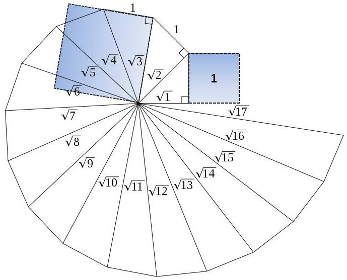
The Spiral of Theodorus is used as the geometric guardrail. It is a spiral figure created by connecting a sequence of right triangles. It begins with an isosceles right triangle with legs of length 1, and each subsequent triangle is built on the hypotenuse of the previous one.
The spiral geometry encodes a fundamental duality between two distinct properties of the universe, which we define as the Matter (Integer) Domain and the Radiation (\(\sqrt{\text{Integer}}\)) Domain.
Philosophy: This separation explains the scaling differences observed in cosmology. Mass density (\(\propto 1/t_{age}^2\)) resides in the circumference (Integer) domain, while CMB temperature (\(\propto 1/\sqrt{t_{age}}\)) resides in the radius (Radiation) domain. The interaction between these domains is mediated by the sqrt of Planck momentum \(\sqrt{kg \cdot m/s}\)—which serves as the link between the integer and \(\sqrt{\text{integer}}\) domains.
Note: As there is no baryonic matter included in this discussion, the CMB peak frequency \(f_{peak} = 160.2\,\text{GHz}\) is used to determine a value for number of increments \(t_{age}\) until ‘now’.
Hawking temperature \(T\) for a Schwarzschild (non-rotating, uncharged) black hole is given by
\[ T = \frac{h c^3}{32 \pi^2 G M k_B} \]If we replace M with Planck mass \(m_P\) then we can re-define \(T\) in terms of Planck temperature \(T_p\) (\(A\) is an Ampere).
\[ T_p = \frac{A c}{2 \pi},\qquad G = \frac{c^2 l_p}{m_P},\qquad h = 2 \pi m_P c l_p,\qquad k_B = \frac{2 \pi c m_P}{A} \] \[ T = \frac{h c^3}{32 \pi^2 G m_P k_B} = \frac{T_p}{8 \pi} \]According to the spiral framework, temperature is considered as a radiation parameter and so follows the spiral radius whereby the temperature drops according to the sqrt of \(t_{age}\) (1, \(\sqrt{2}\), \(\sqrt{3}\), ...). Therefore the temperature of the Planck lattice would be a function of (the sqrt of) time:
\[ T_{cmb} = \frac{T_p}{8 \pi \sqrt{t_{age}}} \]Inserting \(T_{cmb}\) in the following
\[ \frac{x e^x}{e^x-1} - 3 = 0,\qquad x = 2.82143937\ldots \] \[ \frac{k_B T_p}{h} = \frac{1}{2 \pi t_p} \] \[ f_{peak} = \frac{k_B T_{cmb} x}{h} = \frac{x}{8 \pi^2 \sqrt{t_{age}} \cdot 2 t_p} \]If \(f_{peak} = 160.2\,\text{GHz}\) then \(t_{age} = 0.42807 \times 10^{61}\).
Giving present universe age = \(0.42807 \times 10^{61}\, t_p\).
In years this is 6% higher than the observed CMB (13.8 billion yrs):
The mass/length domain resides in the spiral length
\[ t_p = \frac{l_p}{c}\;\text{(s)},\qquad m_{cmb} = (2 t_{age}) m_P = 0.1863589 \times 10^{54}\;\text{kg} \] \[ v_{cmb} = \frac{4 \pi r^3}{3} = 0.8875035 \times 10^{80}\;\text{m}^3,\qquad r = (2 t_{age}) \cdot 2 l_p = 2 c t_{sec} = 0.2767115 \times 10^{27}\;\text{m} \] \[ \frac{m_{cmb}}{v_{cmb}} = \frac{3 m_P}{4 \pi (2 t_{age})^2 (2 l_p)^3} = 0.20998 \times 10^{-26}\;\left(\frac{\text{kg}}{\text{m}^3}\right) \]Via the Friedman equation, replacing \(\rho\) with the above mass density formula reduces to (\(G = c^2 l_p/m_P\)):
\[ \lambda = \frac{3 c^2}{8 \pi G \rho} = (2 c t_{sec})^2 = r^2 \]Dark matter density: \(\rho_{dm} = \Omega_{cdm} \rho_c = 0.265 \times 8.52 \times 10^{-27} = 0.224 \times 10^{-26}\,\text{kg/m}^3\) [9].
Note 1. The mass/density calculated here uses only Planck mass and Planck length without any baryonic matter, yet at \(0.21 \times 10^{-26}\) it compares closely with the observed dark matter density (within 6%). If dark matter is not baryonic then such a close correlation is worth examining.
Note 2. To equate with the CMB radius of the universe our radius requires an additional \(2\pi\) term: \(r_l = 2\pi r = 2\pi (t_{age}) \cdot 2 l_p = 8.7 \times 10^{23}\,\text{km}\).
The mass/volume formula (Matter Domain) uses \(t_{age}^2\), while the temperature formula (Radiation Domain) uses \(\sqrt{t_{age}}\). We may therefore eliminate the age variable \(t_{age}\) and combine both formulas into a single constant of proportionality that resembles the radiation density constant.
\[ T_p = \frac{m_P c^2}{k_B} = \sqrt{\frac{h c^5}{2\pi G {k_B}^2}} \] \[ \frac{m_{cmb}}{v_{cmb} T_{cmb}^4} = \frac{2^5 \cdot 3 \pi^3 m_P}{l_p^3 T_P^4} = \frac{2^8 \cdot 3 \pi^6 k_B^4}{h^3 c^5} \]From Stefan Boltzmann constant \(\sigma_{SB}\)
\[ \sigma_{SB} = \frac{2 \pi^5 k_B^4}{15 h^3 c^2} \] \[ \frac{4\sigma_{SB}}{c} \cdot T_{cmb}^4 = \frac{c^2}{1440 \pi} \cdot \frac{m_{cmb}}{v_{cmb}} = 0.417166 \times 10^{-13} \]The Casimir force per unit area for idealized, perfectly conducting plates with vacuum between them, where \(d_c \cdot 2 l_p\) = distance between plates in units of Planck length:
\[ \frac{-F_c}{A} = \frac{\pi h c}{480 {(d_c \cdot 2 l_p)}^4} \]If \(d_c = 2 \pi \sqrt{t_{age}}\) then eq. (17) = eq. (18), equating the Casimir force with the background radiation energy density and the spiral circumference.
\[ \frac{\pi h c}{480 {(d_c \cdot 2 l_p)}^4} = \frac{c^2}{1440 \pi} \cdot \frac{m_{cmb}}{v_{cmb}} \]Note: This connection defines the Casimir force as a Radiation Domain phenomenon. Article 7 extends this to the atomic scale, showing that both macroscopic Casimir forces and atomic binding energies arise from vacuum polarization along the perpendicular \(w\)-axis dimension, scaling as \(1/r^4\).
\(r_c = 2 \pi \sqrt{t_{age}} \cdot 2 l_p = 0.000420\,\text{m}\) (present Casimir distance).
Compares with \(r_l = 2\pi (t_{age}) \cdot 2 l_p\) (radius of the universe).
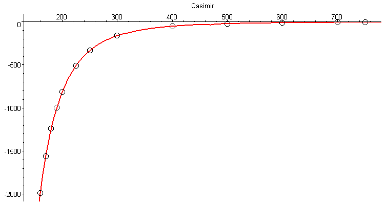
Fig. 1 plots Casimir length \(d_c \cdot 2 l_p\) against radiation energy density pressure measured in mPa for different \(t_{age}\) with a vertex around 1Pa.
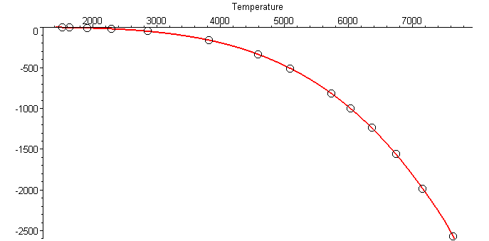
Fig. 2 plots temperature \(T_{cmb}\). A radiation energy density pressure of 1Pa gives \(t_{age} \sim 0.8743 \times 10^{54} t_p\) (2987 years), length = 189.89 nm and temperature \(T_{cmb} = 6034\,\text{K}\).
In conventional units \(0.21668 \times 10^{-17}\) translates to 66.861
\[ H = \frac{1}{2 t_{age} t_p} = 0.21668235 \times 10^{-17}\,\text{s}^{-1} \]Riess and Perlmutter (notes) using Type 1a supernovae calculated the end of the universe \(t_{end} \sim 1.7 \times 10^{-121} \sim 0.588 \times 10^{121}\) units of Planck time:
\[ t_{end} \sim 0.588 \times 10^{121} \]The maximum temperature \(T_{max}\) would be when \(t_{age} = 1\). What is of equal importance is the minimum possible temperature \(T_{min}\) – that temperature 1 Planck unit above absolute zero, for in the context of this model, this temperature would signify the limit of expansion (the black-hole could expand no further). For example, if we simply set the minimum temperature as numerically the inverse of the maximum temperature then:
\[ T_{min} \sim \frac{1}{T_{max}} \sim \frac{8 \pi}{T_P} \sim 0.177 \times 10^{-30}\,\text{K} \]Reversing eq. (3)
\[ 0.177 \times 10^{-30}\,\text{K} = \frac{T_p}{8 \pi \sqrt{t_{age}}} \]Gives
\[ t_{age} = \left(\frac{T_p}{8 \pi}\right)^4 = 1.014 \times 10^{123} \]This would then give us a value ‘the end’ in units of Planck time (\(\sim 0.35 \times 10^{73}\) yrs) which is close to Riess and Perlmutter:
\[ t_{end} \sim 1.014 \times 10^{123} t_p \]The mid way point (\(T_{mid} = 1\,\text{K}\)) becomes \(T_{max}^2 \sim 3.18 \times 10^{61} \sim 108.77\) billion years.
Note: ... in 1998, two independent groups, led by Riess and Perlmutter used Type 1a supernovae to show that the universe is accelerating. This discovery provided the first direct evidence that \(\Omega\) is non-zero, with \(\Omega \sim 1.7 \times 10^{-121}\). This remarkable discovery has highlighted the question of why \(\Omega\) has this unusually small value. So far, no explanations have been offered for the proximity of \(\Omega\) to \(1/{t_u}^2 \sim 1.6 \times 10^{-122}\), where \(t_u \sim 8 \times 10^{60}\) is the present expansion age of the universe in Planck time units. Attempts to explain why \(\Omega \sim 1/{t_u}^2\) have relied upon ensembles of possible universes, in which all possible values of \(\Omega\) are found [11].
[1] Macleod, Malcolm J. "The Programmer God, are we in a simulation?" theprogrammergod.com
[2] Macleod, M.J. Programming Planck units from a virtual electron: a simulation hypothesis. Eur. Phys. J. Plus 133, 278 (2018). https://doi.org/10.1140/epjp/i2018-12094-x
[3] Macleod, Malcolm J., 1. Planck unit scaffolding to Cosmic Microwave Background correlation https://www.doi.org/10.2139/ssrn.3333513
[4] Macleod, Malcolm J., 2. Relativity as the mathematics of perspective in a hyper-sphere universe https://www.doi.org/10.2139/ssrn.3334282
[5] Macleod, Malcolm J., 3. Gravitational orbits from n-body rotating particle-particle orbital pairs https://www.doi.org/10.2139/ssrn.3444571
[6] Macleod, Malcolm J., 4. Geometrical origins of quantization in H atom electron transitions https://www.doi.org/10.2139/ssrn.3703266
[7] Macleod, Malcolm J., 5. Atomic Transitions via a Photon-Orbital Hybrid https://www.doi.org/10.13140/RG.2.2.10680.20487
[8] Macleod, Malcolm J., 6. Do these anomalies in the physical constants constitute evidence of coding? https://www.doi.org/10.2139/ssrn.4346640
[9] Macleod, Malcolm J., 7. Geometric Origin of Quarks, the Mathematical Electron extended https://www.doi.org/10.13140/RG.2.2.21695.16808
[10] Macleod, Malcolm J., 8. Holographic Emergence in the Simulation Hypothesis https://www.doi.org/10.13140/RG.2.2.20919.28320
[11] Planck Collaboration (2020), Planck 2018 results. VI. Cosmological parameters Astronomy and Astrophysics, 641, A6. arXiv:1807.06209
[12] D. J. Fixsen (COBE/FIRAS analyses) and J. C. Mather et al. (COBE) for the precise CMB monopole temperature.
[13] J. Barrow, D. J. Shaw; The Value of the Cosmological Constant arXiv:1105.3105v1 [gr-qc] 16 May 2011
[14] Egan C.A, Lineweaver C.H; A LARGER ESTIMATE OF THE ENTROPY OF THE UNIVERSE; https://arxiv.org/pdf/0909.3983v3.pdf